4.18 Electron excitation analysis
Main function 18 of Multiwfn is very powerful, it is a collection of electron excitation analysis methods and able to provide very deep insight into all aspects of electron transition characters. In this section I will illustrate most of them using practical instances. Before following the examples below, please at least first read beginning of Section 3.21 to understand requirement on the input files. Although I illustrate all analyses based on files generated by Gaussian, these analyses are by no means limited to Gaussian users! Most analyses illustrated in this section (e.g. hole-electron analysis) require orbital wavefunctions of reference state and configuration coefficients, if you are an ORCA user and want to perform these analyses, I highly suggest reading my blog article “Method of performing hole-electron and relevant analyses via Multiwfn in combination with TDDFT calculation of ORCA” (http://sobereva.com/758, in Chinese).
4.18.1 Using hole-electron analysis to fully characterize electron excitations
The hole-electron analysis module of Multiwfn is quite powerful, it is able to present very comprehensive characterization for all kinds of electron excitations. If you are not familiar with basic theories and ideas of hole-electron analysis, please read Section 3.21.1. The requirement on input file for the hole-electron analysis has been described at the beginning of Section 3.21, please carefully check it. Below I will employ two systems to illustrate the use of the hole-electron analysis, the first one is a typical donor-π-acceptor system, the second one is a typical coordinate. The Chinese version of this section is my blog article "Using Multiwfn to perform hole-electron analysis to fully investigate electronic excitation character" (http://sobereva.com/434), in which there is an additional example, namely studying Rydberg excitation of H2CO.
If hole-electron is employed in your work, please not only cite Multiwfn original paper but also cite my work: Carbon, 165, 461 (2020) DOI: 10.1016/j.carbon.2020.05.023, in which hole-electron analysis is briefly described in supplemental information.
4.18.1.1 Example 1: NH2-biphenyl-NO2
The example in this section is quite long, please carefully and patiently read it. In this section I will take the NH2-biphenyl-NO2 as example, its geometry is shown below.
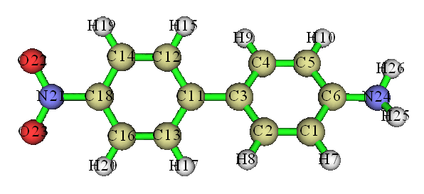
In this system the biphenyl moiety behaves as a π-linker, and it is well-known that the nitro group and amino group act as electron acceptor and donor during electron excitation, respectively, therefore it is expected that there must be some charge-transfer (CT) states corresponding to overall electron displacement from the amino group side to the nitro group side.
Preparation
Here I assume that you are a Gaussian user (other quantum chemistry codes users can also utilize the hole-electron analysis). We optimize the geometry at the B3LYP/6-31G* level, then carry out TDDFT calculation using below settings (the input file has been provided as examples\excit\D-pi-A.gjf), then five lowest singlet excited states will be evaluated. Note that IOp(9/40=4) must be specified, the reason has been clearly mentioned at the beginning of Section 3.21. The CAM-B3LYP is employed here because it is able to faithfully represent CT excitations.
%chk=D-pi-A.chk
# CAM-B3LYP/6-31g(d) TD(nstates=5) IOp(9/40=4)
After calculation, convert the .chk file to .fch/fchk file, the resulting .fchk file has been provided as examples\excit\D-pi-A.fchk. The output file of this task has been provided as examples\excit\D-pi-A.out.
Examining quantitative indices defined in the hole-electron analysis framework
Boot up Multiwfn and input the following commands
examples\excit\D-pi-A.fchk
18 // Electron excitation analysis
1 // Hole-electron analysis
examples\excit\D-pi-A.out // In fact you can also press ENTER button directly, because the name of the .out file is identical to the .fchk file and they are in the same folder
1 // Study excitation between ground state (S0) and the first excited state (S1)
1 // Calculate distribution of hole, electron and so on as well as various indices
2 // Medium-quality grid (this is suited for small and medium sized systems. For large systems, you should use at least "high-quality grid", or manually input a proper grid spacing)
Once calculation is finished, you will find the following information on screen. The data (except for the excitation energy) are calculated by grid-based integration. Clearly, for the same system, the higher number of grids, the better accuracy of the data.
 Integral of hole:        1.000343
 Integral of electron:    0.999793
 Integral of transition density:   -0.000033
 Transition dipole moment in X/Y/Z:   0.444063  -0.000186  -0.001753 a.u.
 Sm index (integral of Sm function):   0.27369 a.u.
 Sr index (integral of Sr function):   0.51896 a.u.
 Centroid of hole in X/Y/Z:       -4.531729    0.000425    0.003252 Angstrom
 Centroid of electron in X/Y/Z:   -4.010033    0.001760    0.002643 Angstrom
 D_x:   0.522  D_y:   0.001  D_z:   0.001    D index:   0.522 Angstrom
 Variation of dipole moment with respect to ground state:
 X:   -0.985930  Y:   -0.002523  Z:    0.001150    Norm:    0.985934 a.u.
 RMSD of hole in X/Y/Z:       1.443   1.160   0.437   Norm:   1.902 Angstrom
 RMSD of electron in X/Y/Z:   1.596   0.974   0.634   Norm:   1.974 Angstrom
 Difference between RMSD of hole and electron (delta sigma):
 X:  0.153  Y: -0.186  Z:  0.197    Overall:  0.072 Angstrom
 H_x:  1.520  H_y:  1.067  H_z:  0.536  H_CT:  1.520  H index:  1.938 Angstrom
 t index: -0.998 Angstrom
 Hole delocalization index (HDI):      22.68
 Electron delocalization index (EDI):  17.11
 Ghost-hunter index:    -18.831 eV, 1st term:  8.771 eV, 2nd term:    27.601 eV
 Excitation energy of this state:     3.907 eV
In the output, the "Integral of hole" and "Integral of electron" are the integrals of hole and electron over the whole space, respectively, they should be exactly 1.0 in principle. However, due to the unavoidable numerical integration error, the calculated values have slight deviation to 1.0. Since the deviation is extremely small, we can say that for the current excited state of the current system, the grid setting we employed is fully adequate.
Note
If you find the integral of hole or electron deviates from 1.0 evidently, then the outputted indexes may be unreliable. There are three possibilities: (1) You forgot to use IOp(9/40=3 or 4) (2) The grid quality is too low (3) The extension distance is not large enough, therefore the spatial region of the grid points does not fully cover the main distribution region of hole or electron (when Rydberg excitation is investigated, the default extension distance should always be enlarged).
The rest terms in the above output in turn are: The integral of transition density over the whole space (ideal value is 0), transition electric dipole moment, \(S_{\mathrm{m}}\) and \(S_{\mathrm{r}}\) indices, centroid coordinate of hole and electron, Dλ and D indices, X/Y/Z components and norm of variation of excited state dipole moment with respect to the ground state one, RMSD (σ) of hole and electron, Δσλ and Δσ indices, Hλ/\(H_{\mathrm{CT}}\)/H indices, t index, hole and electron delocalization index, Ghost-hunter index, excitation energy (which is loaded from Gaussian output file directly).
Note
Note that the "Ghost-hunter index" in above output is slightly different to the definition in its original paper, the implementation in Multiwfn must be more reasonable, see Section 3.21.7 for detail. The 1st term denotes the part depending on configuration coefficients and MO energies, while the 2nd term corresponds to 1/D. The ghost-hunter index is just the difference of the two terms.
The transition dipole moment outputted above is obtained by integrating evenly distributed grids of transition dipole moment density. It can also be directly read from the Gaussian output file, the X/Y/Z components are 0.4427, -0.0005, -0.0012 a.u., which are very close to those outputted by Multiwfn, namely 0.444063, -0.000186, -0.001753. This observation further reflects that the grid setting we employed is appropriate.
For the S0→S1 excitation under current study, from the above output, it can be seen that the D index is merely 0.522 Å, which is obviously a very small value since it is even less than half length of a typical C-C bond. The \(S_{\mathrm{r}}\) index reaches 0.519 (the theoretical upper limit is 1.0), which is a large value, implying that about half part of hole and electron have perfectly matched. So, by simply examining \(S_{\mathrm{r}}\) and D indices, we are already able to conclude that this excitation should be a typical local excitation (LE). Then let us look at the t index, its total value is -0.998, which is much less than 0, meaning that there is no significant separation of hole and electron distributions, further implying that this excitation should be attributed to LE type.
Visual study of various real space functions in the hole-electron framework
Now you should see the post-processing menu on the screen. The meaning of each option is self-explanatory. Please read through each option carefully. Here we choose option 3, we will see distribution of hole and electron at the same time:
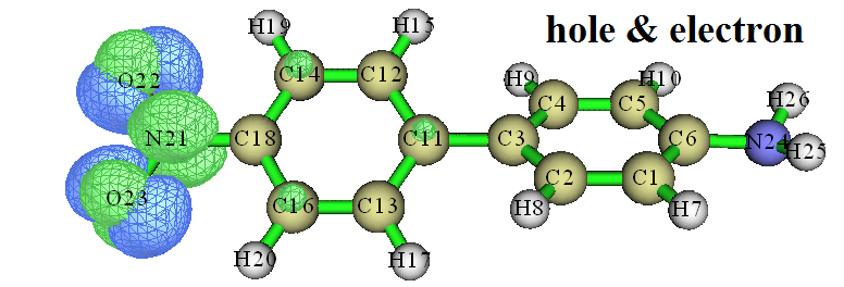
In above figures, green represents the electron distribution, and blue represents the hole distribution, isovalue has been set to 0.005. Both the hole and electron appear almost exclusively in the nitro group, so there is no doubt that S0→S1 is a LE excitation, well verifying our conclusion based on the D, \(S_{\mathrm{r}}\), and t indices. In addition, according to the above hole distribution map, the hole appears to be composed of lone pair orbitals of oxygens since there is one lobe on each side of each oxygen. Electron distribution has a nodal plane along the nitro group, therefore we can infer that the electron distribution should be composed of π* orbital. Now we can draw the conclusion that that S0→S1 is a LE excitation with n→π* feature.
Then close the graphical window and select option 8 to visualize \(C_{\mathrm{hole}}\) and \(C_{\mathrm{ele}}\), which are transformed from hole and electron distributions respectively to make their distribution behavior smoother. The isosurface map is shown below (In order to see clearly, transparent style is used).
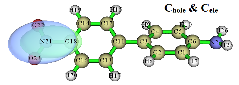
As can be seen, the graph of \(C_{\mathrm{hole}}\) and \(C_{\mathrm{ele}}\) look obviously more intuitive, they are very sleek and do not have any nodal character like hole and electron. Therefore, using \(C_{\mathrm{hole}}\)/\(C_{\mathrm{ele}}\) map to replace the hole/electron map is a good choice in many cases. (BTW: If isosurfaces of \(C_{\mathrm{hole}}\) and \(C_{\mathrm{ele}}\) are not visible in the GUI window, that means the current isovalue is too large, you should gradually and carefully decrease it until the isosurfaces are visible)
Next, let us take a look at the overlap function of hole and electron, namely the \(S_{\mathrm{r}}\) function. Close current graphical window, select option 4 in the post-processing menu, and then select option 2 to display the \(S_{\mathrm{r}}\) function, you will see the map below (isovalue is set to 0.005)
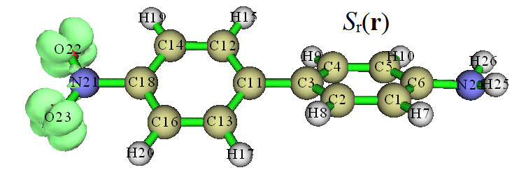
From the graph one can clearly find where the hole and electron overlap significantly. As can be seen, around each oxygen there are four regions where the hole and electron are highly overlapped. It is easy to understand why the \(S_{\mathrm{r}}\) graph looks like this by comparing the hole and electron isosurfaces shown earlier.
Then close the window and select option 7, charge density difference (CDD) between the excited state and the ground state will be shown, see below. In this map, the isovalue is set to 0.005, green and blue correspond to increase and decrease of the excited state density with respect to the ground state density, respectively.
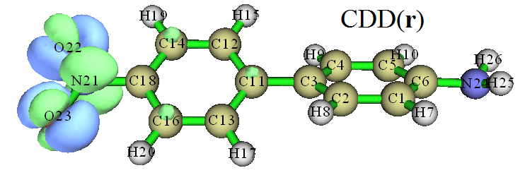
The CDD map and the map simultaneously showing hole and electron distributions (referred to as "hole&electron map" later) are similar with each other, but there are also differences. The key difference is that in the CDD map, the hole and electron have been largely cancelled in their overlapping region; in contrast, in the hole&electron map, the overlapping between hole and electron can be faithfully exhibited. I think the hole&electron map is more useful than the CDD map to investigate the intrinsic characteristics of electron excitation because it directly exhibits the pristine distribution of hole and electron.
By the way, if we select option 18 in the post-processing menu, the program will start to calculate the Coulomb attractive energy (also known as exciton binding energy) between the hole and electron. The calculation is quite time-consuming even for medium sized system, so please wait patiently. The final output is:
Important note: By using VMD software, you can plot above-mentioned functions of much better quality with only a few steps. I strongly suggest you check the example given in Section 4.A.14 on how to do this.
Examining quantitative contributions to hole and electron
Next, I will demonstrate how to evaluate contribution of MOs to hole and electron. After selecting option 0 in the post-processing menu to return to the hole-electron analysis interface, we select subfunction 2 and input an outputting threshold. Here we input 1, then MOs with contribution to hole or electron higher than 1% will be shown on screen:
 MO   52, Occ:   2.00000    Hole:   96.207 %    Electron:    0.000 %
 MO   56, Occ:   2.00000    Hole:    3.415 %    Electron:    0.000 %
 MO   57, Occ:   0.00000    Hole:    0.000 %    Electron:   85.411 %
 MO   59, Occ:   0.00000    Hole:    0.000 %    Electron:   12.222 %
 MO   61, Occ:   0.00000    Hole:    0.000 %    Electron:    2.163 %
 Sum of hole:  100.001 %    Sum of electron:  100.001 %
It can be seen from the data that MO52 is absolutely dominant for hole, it contributes as high as 96.2%, while electron is mainly composed of MO57, with a contribution of 85.4%. This observation implies that if one discusses electron excitation solely based MO52 and MO57, although in this case the electron excitation can be qualitatively described, there are still non-negligible deviations. The "Sum of hole" and "Sum of electron" shown above are the sum of the contributions of all orbitals to hole and electron, respectively (including the terms not outputted), these two values in principle should be exactly 100%, but currently there are 0.001% error. Such a small error can be completely ignored, it comes from the fact that not all configuration coefficients are printed by Gaussian (only configuration coefficients greater than 0.0001 are requested to be outputted during Gaussian calculation via IOp(9/40=4)).
Then we check contribution of atoms or fragments to hole and electron. Select subfunction 3 in hole-electron analysis interface, then choose Mulliken-like partition, you will see
 The number of non-hydrogen atoms:        16
 Contribution of each non-hydrogen atom to hole and electron:
    1(C )  Hole:  0.19 %  Electron:  0.02 %  Overlap:  0.07 %  Diff.:  -0.17 %
    2(C )  Hole:  0.18 %  Electron:  0.48 %  Overlap:  0.30 %  Diff.:   0.30 %
    3(C )  Hole:  0.59 %  Electron:  0.13 %  Overlap:  0.28 %  Diff.:  -0.46 %
    4(C )  Hole:  0.18 %  Electron:  0.49 %  Overlap:  0.30 %  Diff.:   0.32 %
    5(C )  Hole:  0.19 %  Electron:  0.02 %  Overlap:  0.06 %  Diff.:  -0.18 %
    6(C )  Hole:  0.31 %  Electron:  0.37 %  Overlap:  0.34 %  Diff.:   0.06 %
   11(C )  Hole:  0.15 %  Electron:  4.17 %  Overlap:  0.78 %  Diff.:   4.03 %
   12(C )  Hole:  0.41 %  Electron:  0.14 %  Overlap:  0.24 %  Diff.:  -0.26 %
   13(C )  Hole:  0.37 %  Electron:  0.14 %  Overlap:  0.23 %  Diff.:  -0.23 %
   14(C )  Hole:  0.94 %  Electron:  5.03 %  Overlap:  2.18 %  Diff.:   4.09 %
   16(C )  Hole:  0.92 %  Electron:  5.01 %  Overlap:  2.15 %  Diff.:   4.09 %
   18(C )  Hole: -0.01 %  Electron:  1.16 %  Overlap:  0.00 %  Diff.:   1.17 %
   21(N )  Hole:  2.39 %  Electron: 33.90 %  Overlap:  9.00 %  Diff.:  31.52 %
   22(O )  Hole: 46.18 %  Electron: 24.38 %  Overlap: 33.55 %  Diff.: -21.80 %
   23(O )  Hole: 46.12 %  Electron: 24.39 %  Overlap: 33.54 %  Diff.: -21.73 %
   24(N )  Hole:  0.46 %  Electron:  0.15 %  Overlap:  0.26 %  Diff.:  -0.32 %
Since hydrogen atoms generally do not participate in electron excitation of chemical interest, only the information of non-hydrogen atoms is outputted, including the atomic contributions to hole, electron, hole-electron overlap, electron-hole difference (i.e. CDD). The indices of the atoms in the nitro group are 21, 22, and 23, it can be seen from the data that the two oxygens of the nitro group contribute most to the hole, the sum of their contributions is 2×46.1≈92%. The spatial delocalization of the electron is relatively stronger, the three atoms in the nitro group contribute a total of 2×24.4+33.9≈83%, the rest part of electron is basically contributed by the atoms in the biphenyl moiety.
Although the distribution characteristics of hole and electron can be examined by visualizing isosurface map of hole and electron, the observed isosurfaces are obviously dependent on the choice of isovalue. So, it is impossible to fully display the hole and electron distribution in all regions by only one image. On the contrary, the quantitative atomic contributions given above are very definitive.
The sum of "Diff." of N21, O22 and O23 is about -12%, which shows that the integral value of the density difference (CDD) in the nitro group is -0.12, revealing that the nitro moiety lost 0.12 electrons during electron excitation, and some of them transferred to the biphenyl moiety (if you want to investigate charge transfer amount between specific fragments, it is recommended to use the IFCT method, as illustrated in Section 4.18.8).
Showing atomic contributions to hole and electron in terms of heat map
We can also plot the atomic contributions as heat map, so that the major character can be immediately and easily captured. Select "4 Set interval between labels in X axis" in current menu and then input 1 to change the step of abscissa to 1, and then select "1 Plot hole/electron composition as heat map", you will see the map below immediately

In the figure, the numbers in the abscissa are indices of non-hydrogen atoms. This figure describes the contribution of each non-hydrogen atom to hole, electron and their overlap by color (e.g. 0.4 corresponds to 40%). For example, based on the list of contributions of non-hydrogen atoms to hole/electron that shown earlier, we can know that the position 16 in the abscissa of the figure actually corresponds to atom N24. In order to more conveniently find the correspondence between the indices in the abscissa and actual atomic indices, you can open corresponding .fch/.gjf/.out file by GaussView, Select "Edit" - "Atom List", then select "Edit" - "Reorder" - "All atoms: Hydrogens Last", then you will see the graph below in GaussView, in which indices of all hydrogen atoms have been placed behind indices of non-hydrogen atoms. Clearly, in this case the atomic indices in the molecular structure directly correspond to the indices in the abscissa of the heat map.
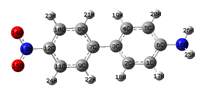
From indices in the map above, we find that the positions of 13, 14 and 15 in the heat map correspond to the two oxygens and one nitrogen atoms in the nitro group, the position 16 corresponds to the nitrogen in amino group, the rest are carbons in the biphenyl moiety. In the heat map, the row corresponding to hole clearly revealed that the hole is almost solely contributed by the two oxygens in the nitro group, since corresponding matrix elements are red (large value). Electron is also mainly contributed by the nitro group, but other molecule regions also have non-negligible contributions, this is why in the row corresponding to electron, blue color appears in the matrix elements other than positions 13~15. The information conveyed by colors of the row corresponding to overlap is that there is significant overlap between hole and electron on the oxygens of the nitro groups, while the overlap in other areas of the systems is far from being so remarkable.
There are many options in the hole/electron composition analysis interface, they can be used to adjust plotting effect of the heat map, save the heat map as an image file, switch whether to include the hydrogen atoms into the heat map, and export the data to he_atm.txt in current folder so that you can draw the heat map yourself in other programs such as Origin. These options will not be explained one by one here, please try it yourself.
Investigating fragment contributions to hole and electron
The option "-1 Load fragment definition" in the above hole/electron composition analysis interface is important, it is used to load fragment definition, then fragment contribution to hole and electron will be shown, and fragment-based heat map could be drawn, which makes the discussion significantly more convenient. Here we divide the system into four fragments in the following way.
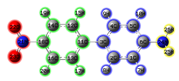
Select option "-1 Load fragment definition", and then input
4 // Define four fragments
21-23 // The atomic indices of fragment 1 (the nitro group)
11-20 // The atomic indices of fragment 2 (the benzene neighbouring to nitro group)
1-10 // The atomic indices of fragment 3 (the benzene neighbouring to amino group)
24-26 // The atomic indices of fragment 4 (the amino group)
You will see below output immediately
  Contribution of each fragment to hole and electron:
 #  1   Hole: 94.68 %  Electron: 82.67 %  Overlap: 88.47 %  Diff.: -12.01 %
 #  2   Hole:  3.20 %  Electron: 15.67 %  Overlap:  7.09 %  Diff.:  12.47 %
 #  3   Hole:  1.64 %  Electron:  1.53 %  Overlap:  1.59 %  Diff.:  -0.12 %
 #  4   Hole:  0.47 %  Electron:  0.13 %  Overlap:  0.25 %  Diff.:  -0.34 %
The data shows that 94.68% of hole is located on the nitro group, while 82.67% and 15.67% of electron are located on the nitro group and neighbouring benzene ring, respectively. The degree of overlap between hole and electron on the nitro group is about 90%. Since "Diff." of the nitro group is -12.01%, and the excitation under current investigation is a single electron excitation, therefore, it can be said that the electron on the nitro group is reduced by 0.1201 during the electron excitation process, while the benzene ring neighbouring to the nitro group gained 0.1247 electrons. Then, if you want to make representation of the above data more intuitive, we can select option 1 to draw the fragment-based heat map. The abscissa at this time corresponds to fragment index, as shown below:
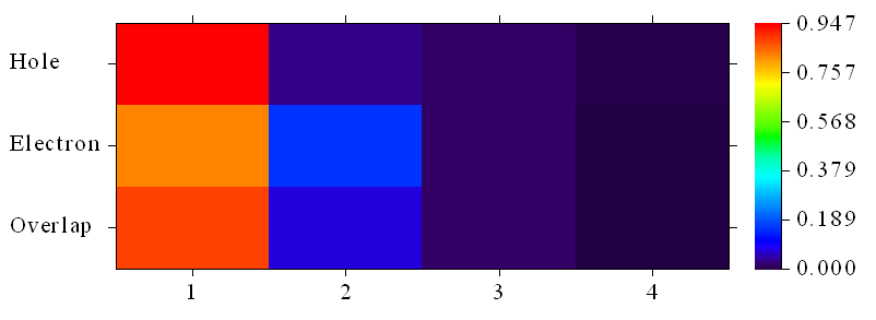
It can be seen from the figure that the spatial distribution range of electron is larger than hole.
Collective comparison of all electron excitations
At this point, various analyses in the hole-electron framework for the S0→S1 excitation of the NH2-biphenyl-NO2 system have been completely completed. If you also want to analyze other excited states, you should return to the menu of main function 18 by option 0, enter the hole-electron analysis function again, and then select the corresponding excited state. Here we put together the D, \(S_{\mathrm{r}}\), H, t index and hole-electron Coulomb attraction energy of all the five excited states calculated in this system. The hole delocalization index (HDI) and electron delocalization index (EDI), which have not been discussed earlier, are also given:
| D(Å) | Sr | H(Å) | t(Å) | Ecoul(eV) | HDI | EDI | |
|---|---|---|---|---|---|---|---|
| S0→S1 | 0.52 | 0.52 | 1.94 | -1.00 | 7.81 | 22.7 | 17.1 |
| S0→S2 | 3.48 | 0.65 | 3.15 | 0.56 | 4.71 | 7.2 | 9.5 |
| S0→S3 | 0.57 | 0.55 | 1.70 | -0.68 | 8.54 | 19.7 | 17.2 |
| S0→S4 | 0.97 | 0.87 | 2.88 | -1.55 | 5.56 | 7.0 | 7.0 |
| S0→S5 | 0.54 | 0.87 | 2.93 | -2.06 | 5.56 | 6.9 | 7.1 |
The following maps are hole&electron map, \(C_{\mathrm{hole}}\)&\(C_{\mathrm{ele}}\) map and \(S_{\mathrm{r}}\) function map of all the five excitations. The isovalues are set to 0.003 a.u. It can be seen that the \(C_{\mathrm{hole}}\)&\(C_{\mathrm{ele}}\) map can always display the main distribution features of the hole&electron map in a clearer and more intuitive way. However, many details are lost during the transformation; for example, it is impossible to determine the specific type of the electron excitation (such as n-π*, π-π*) solely based on the \(C_{\mathrm{hole}}\)&\(C_{\mathrm{ele}}\) map.
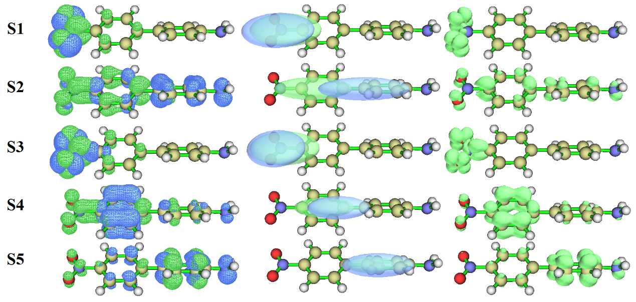
Now we look at the indices together with the isosurface graphs. For the D index, only the S0→S2 value has very large (3.48 Å), so it can obviously be considered as CT excitation. Indeed, from the graph above it can be seen that the distance between the center of the blue and green isosurfaces (namely centroids of \(C_{\mathrm{hole}}\) and \(C_{\mathrm{ele}}\)) is large. While for other excitations, the centers of the blue and green isosurfaces are close together, therefore they should be regarded as LE excitations.
Then we examine the \(S_{\mathrm{r}}\) index. We find that the \(S_{\mathrm{r}}\) indices of all excited states are relatively large. In particular, the values of the S0→S4 and S0→S5 are rather large, up to 0.87, the main reason is that these two excitations are highly localized π-π* type of excitation on the benzene ring. It is worth to mention that although S0→S1 is also a highly localized excitation, its \(S_{\mathrm{r}}\) (0.52) is even smaller than the \(S_{\mathrm{r}}\) (0.65) of S0→S2, which is a CT excitation. The reason why the \(S_{\mathrm{r}}\) index of the S0→S1 is not as large as expectation is not difficult to understand. As mentioned earlier, S0→S1 shows n→π* feature, the main body of lone pair is on the NO2 plane, while π* orbital has a nodal plane on the NO2 plane, hence the overlap of hole and electron should be limited.
Next, look at the H index, which reflects the breadth of the average distribution of hole and electron. It can be seen from the hole&electron map that both the hole and electron of S0→S1 and S0→S3 are distributed in a local region, this is why their H indices are not large. Since the distribution of hole and electron corresponding to the excitations from S0 to S2, S4 and S5 are evidently wider than S0→S1, their H indices are evidently larger.
One can see that only the t index of S0→S2 is a slightly positive value, indicating that the separation of hole and electron is obvious, so it is more reasonable to consider S0→S2 as a CT excitation. The t indices corresponding to the excitations from S0 to other excited states are evident negative values, suggesting that degree of separation of their hole and electron is very low.
By comparing the hole and electron isosurface maps, we can find that the HDI and EDI indices indeed nicely quantified the uniformity of spatial distribution (i.e. degree of delocalization) of hole and electron, respectively. It can be seen that both hole and electron of S0→S1 and S0→S3 are highly localized, corresponding to the calculated large value of HDI and EDI. In contrast, the hole and electron distributions of S0→S2/S4/S5 are evidently more delocalized, this point is faithfully revealed by their relatively small HDI and EDI values.
The hole-electron Coulomb attractive energy given in the table is closely related to the electron excitation characteristics, and the most influential factor should be the D index. It is easy to understand that the larger the D index is, the farther the distance between the main distribution regions of hole and electron, and thus the weaker the Coulomb attractive energy. From the data, it is indeed found that Coulomb attraction energy of S0→S2 (the only CT excitation) is the smallest one of that of all the five electron excitations. While for the excitations of S0→S1 and S0→S3, since their D indices are very small and according to the H index the spatial extent of their hole and electron is very narrow, one can easily imagine that the corresponding Coulomb attraction should be very strong. Indeed, as can be seen from the previous table, their hole-electron Coulomb attraction energies are the most negative ones (-7.81 and -8.54 eV).
Combined with the above isosurface maps and quantitative data, we can unambiguously identify the characteristics of the five excitations:
-
S0→S1:LE excitation of n-π* type on the nitro group
-
S0→S2:CT excitation of π-π* type from amino group towards nitro group
-
S0→S3:The same as S0→S1
-
S0→S4:π-π* LE excitation occurring on the benzene ring attached to the nitro group
-
S0→S5:π-π* LE excitation occurring on the benzene ring attached to the amino group
Here, the heat maps that exhibit contributions to the hole, electron and overlap from all fragments for all the five excitations are given together. In order to facilitate parallel comparison, the color scale for all excited states is uniformly set to 0.0~1.0.
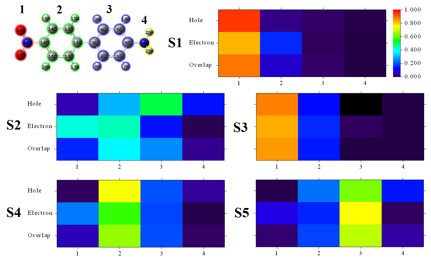
From these heat maps, one can immediately make clear where the excited electrons come and where they go by viewing color of the matrix elements. For example, from the graph of S0→S2, one can easily recognize that the excited electron is mainly originated from fragment 3 (the benzene attached to amino group), most of them is transferred to fragment 1 (the nitro group), and a smaller part is transferred to fragment 2 (the benzene attached to the nitro group). Another example, from the S0→S4 map one can find that the excited electrons come from fragment 2, after excitation most of them remain in fragment 2, but a few of them transferred to fragment 1, and the overlap between hole and electron on fragment 2 is significantly higher than the other regions.
It is worth to note that the detailed characteristics of charge transfer between fragments during electron excitation can be even better revealed by the IFCT method, see example in Section 4.18.8.
Plotting grid data in VMD
The grid data of hole, electron, \(C_{\mathrm{ele}}\), \(C_{\mathrm{hole}}\) and so on can be exported to cube files by corresponding options in the post-processing menu, and then you can render them in VMD program to get better visualization effect. If you do not know how to do, please refer to the description of the operations in VMD at the end of Section 4.18.3. Furthermore, one can first use VMD to plot an isosurface map for \(C_{\mathrm{ele}}\) and \(C_{\mathrm{hole}}\), and then input such as below command to draw centroids of hole and electron as purple and orange spheres to make the graph more informative
draw color purple
draw sphere {1.411500   -0.007015   -0.025494} radius 0.25 resolution 20
draw color orange
draw sphere {-2.069784   -0.000346   -0.000830} radius 0.25 resolution 20
For the S0→S2 excitation, the graph plotted in above way in VMD is shown below
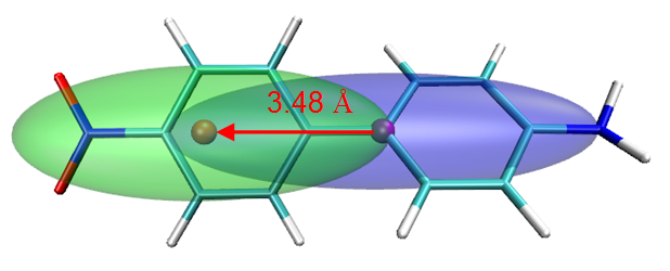
In order to make understanding easier, an arrow is appended on the graph to highlight the CT direction, the D index is also labelled together to make the graph more informative.
Tip: Obtaining a variety of indices for a range of excited states via script
By Linux shell script, a variety of indices for a range of excited states can be obtained at once. For example, we want to obtain all indices for excitations of S0→S1,S2,S3, we should copy the input files D-pi-A.fchk and D-pi-A.out as well as the all_index.sh from the "examples\excit" folder to a proper folder, then enter this folder in the Linux terminal, run chmod +x ./batch.sh to add executable permission, then run ./all_index.sh to execute the script. Each excitation will be analyzed in turn, the status will be shown on screen until the appearance of "Finished!". Then open the resulting result.txt file in current folder, you will find
     1  Sr index (integral of Sr function):   0.51896 a.u.
     2  Sr index (integral of Sr function):   0.64906 a.u.
     3  Sr index (integral of Sr function):   0.54538 a.u.

     1  D_x:   0.522  D_y:   0.001  D_z:   0.001    D index:   0.522 Angstrom
     2  D_x:   3.481  D_y:   0.007  D_z:   0.025    D index:   3.481 Angstrom
     3  D_x:   0.574  D_y:   0.001  D_z:   0.001    D index:   0.574 Angstrom

     1  RMSD of hole in X/Y/Z:       1.443   1.160   0.437   Norm:   1.902 Angstrom
     2  RMSD of hole in X/Y/Z:       3.055   0.826   0.740   Norm:   3.251 Angstrom
     3  RMSD of hole in X/Y/Z:       0.984   1.032   0.416   Norm:   1.486 Angstrom
[ignored...]
This summary of all indices. You can easily modify the script to meet your practical requirement, if you are not familiar with this point, please check Section 5.3.
4.18.1.2 Example 2: Ru(bpy3)2+ cation in water
Below we examine several excited states of the Ru(bpy3)2+ cation complex in water by hole-electron analysis based on TDDFT output.
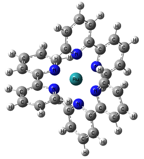
The corresponding Gaussian input file has been provided as examples\excit\Ru(bpy3)2+.gjf, please calculate it by Gaussian. If you want to directly obtain the resulting output file and .fchk file, you can download them at http://sobereva.com/multiwfn/extrafiles/Ru_bpy3_2+_TDDFT.zip. As you can see from the .gjf file, the keywords used are B3LYP/genecp TD(nstates=50) scrf IOp(9/40=3), where scrf requests Gaussian to employ IEFPCM solvation model to represent water environment. Since this system is not small, and as many as 50 excited states are evaluated, in order to avoid too high calculation time in hole-electron analysis and too large Gaussian output file, IOp(9/40=3) is used instead of the IOp(9/40=4) employed in last section, the analysis accuracy at this time is still completely sufficient.
We arbitrarily select three excited states to perform hole-electron analysis, the results are
| D (Å) | Sr | H (Å) | t (Å) | hole (Ru%) | ele (Ru%) | MLCT(%) | |
|---|---|---|---|---|---|---|---|
| S0→S24 | 0.30 | 0.71 | 2.73 | -1.35 | 77.3 | 19.6 | 57.7 |
| S0→S37 | 0.11 | 0.84 | 3.52 | -2.10 | 16.9 | 8.8 | 8.1 |
| S0→S40 | 0.13 | 0.71 | 2.00 | -1.05 | 80.3 | 42.4 | 38.0 |
All D indices in this table are very small, while all \(S_{\mathrm{r}}\) indices are fairly large. The main reason is that the current molecule is a symmetric system, thus the CT transitions are multiple directional. The MLCT(%) in the table denotes percent of metal-to-ligand charge transfer character, which can be easily evaluated in terms of subtracting the percentage of metal in hole (namely hole(Ru%)) by that in electron (namely ele(Ru%)). Notice that, properly speaking, what we obtained is net MLCT percentage, it has been somewhat cancelled with LMCT (ligand-to-metal charge transfer).
Below is hole&electron map of S0→S24 excitation with isovalue of 0.002. Since the hole and electron distributions have a large overlap, for the sake of clarity, the isosurfaces of hole and electron are given separately.
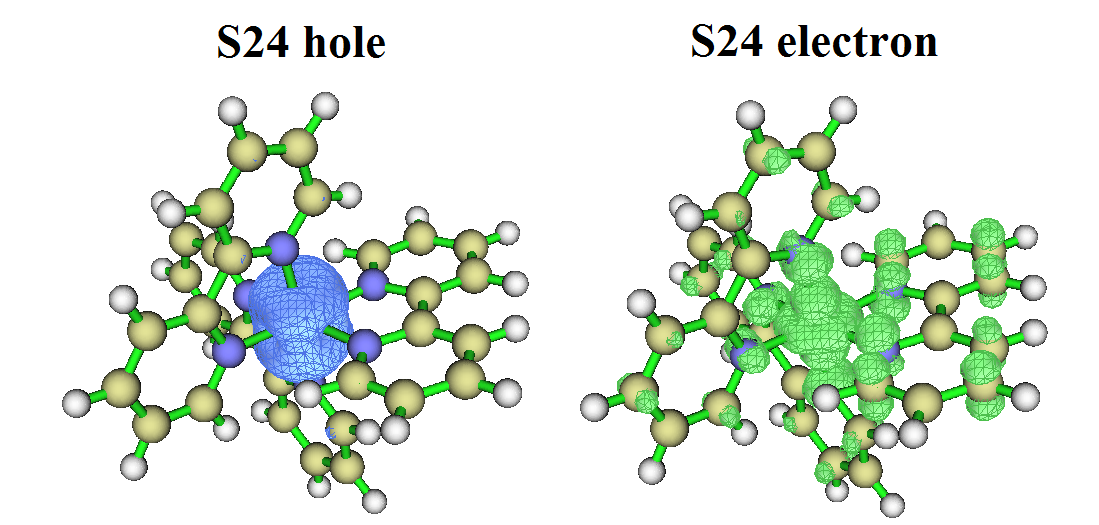
Combining the graph with the quantitative data in the table, it is clear that the S0→S24 excitation not only has metal-centered (MC) character, namely electrons of the metal are excited into the metal's own empty orbital, but also have evident MLCT character. As shown in the hole&electron isosurface map, the main body of both the hole and electron is on the metal, and it can be seen that the isosurface of electron also has a large portion on the ligand. The calculated percentage of MLCT feature is 77.3-19.6 = 57.7%, this value should be said to be very consistent with the information conveyed by the hole-electron isosurface map. Note: The hole also has non-negligible distribution on the ligand, which is 100%-77.3% = 22.7%. The reason why the hole isosurface is invisible on the ligands is because its distribution is very diffuse in this region, the hole on the ligands can only be clearly seen by decreasing the isovalue to a smaller value, such as 0.0005.
Then look at S0→S37 excitation. From the hole&electron isosurface map shown below we can see that main body of both hole and electron is located at one of the ligands, therefore it is no doubt that this is a LC (ligand-centered) excitation, corresponding to the case that electrons excited from ligand to its own π* orbitals. Because there is also hole and electron distribution on the metal, therefore this excitation also shows some MLCT character, which is calculated to be 16.9% - 8.8% = 8.1%.
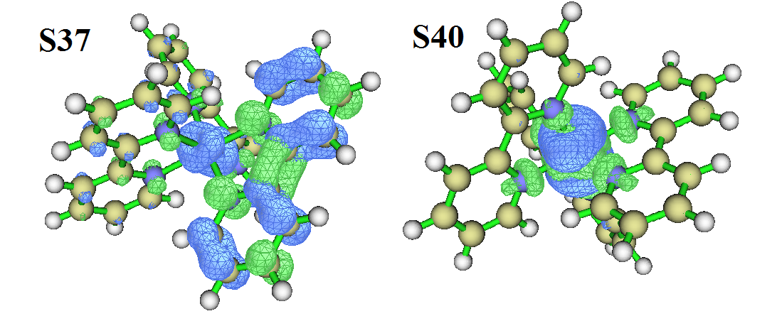
Finally, look at the S0→S40 excitation, whose hole and electron isosurfaces are shown at right part of the map above. From the hole isosurface and the percent of hole on metal shown in the previous table (16.9%), it is found that its hole distribution character is very similar to S0→S24, but the amount of electron on the ligand is obviously not as large as S0→S24, only tiny part of it is distributed on the four nitrogens directly coordinating with Ru, so the MLCT feature of S0→S40 is conspicuously weaker than S0→S24. In contrast, its MC characteristic is definitely higher than S0→S24.
By the way, for coordinate systems, if you want to obtain MLCT, LMCT, LLCT, MC, LC separately, you should resort to the IFCT analysis illustrated in Section 4.18.8.
We already know that the electron in the excitations from S0 to S24 and S40 mainly sources from Ru atoms, but how to unveil which are the atomic orbitals that electron excited from? Although it can be more or less judged from the isosurface map of the hole, there is still some subjectivity. To figure this out, we can calculate contributions of basis functions to hole and electron. For example, after entering the hole-electron analysis function and selecting the 40th excited state, we select "4 Show basis function contribution to hole and electron" and then input an outputting threshold, such as 2, then information of the basis functions contributing to hole or electron higher than 2% will be printed:
   Basis  Type    Atom    Shell     Hole      Electron     Overlap      Diff.
    22    D 0      1(Ru)   12     23.81 %      0.00 %      0.33 %    -23.81 %
    23    D+1      1(Ru)   12      8.90 %     13.63 %     11.01 %      4.72 %
    24    D-1      1(Ru)   12      9.06 %     25.12 %     15.09 %     16.05 %
    25    D+2      1(Ru)   12     13.96 %      6.94 %      9.84 %     -7.02 %
    26    D-2      1(Ru)   12     14.06 %     15.57 %     14.80 %      1.51 %
    27    D 0      1(Ru)   13      3.66 %      0.00 %      0.06 %     -3.66 %
    30    D+2      1(Ru)   13      2.32 %     -0.01 %      0.00 %     -2.32 %
    31    D-2      1(Ru)   13      2.33 %     -0.03 %      0.00 %     -2.35 %
 Sum of above printed terms:      78.10 %     61.22 %                 16.88 %
It can be seen from the data that the main contribution to the hole is the D basis function of the Ru atom. The SDD pseudopotential basis set we currently used only describes 4s, 4p, 4d and 5s electrons for Ru, so the excited electron of S0→S40 excitation must come from the 4d atomic orbitals. The basis functions of Ru that have contributions to electron are also D type. Therefore, now we know that the MC component in the S0→S40 corresponds to d-d transition on Ru.
Note
Notice that this is not the only way to determine which orbitals the excited electrons come from and move to, for example you can also use Multiwfn to perform NTO analysis and examine the pattern of the NTO pair with largest eigenvalue. However, if the electron excitation under study cannot be well described by any pair of NTOs, then this approach will not work. In contrast, the hole-electron analysis does not have any limitation.
4.18.2 Illustration of transition density (matrix) and transition dipole moment density (matrix) analysis
The transition density and transition dipole moment density are very important quantities involved in electron excitation analysis, they can be studied in the form of real space functions by hole-electron module, or studied in Hilbert space by plotting as colored matrix maps (also known as heat maps). The examples in Sections 4.18.2.1, 4.18.2.2 and 4.18.2.3 will illustrate these analyses. In addition, although the commonly studied transitions are those from ground state to excited states, these quantities between two excited states are also useful in some special studies, Section 4.18.2.4 will mention how to realize this.
More discussions about these topics can be found from my blog article: "Using Multiwfn to plot transition density matrix and charge transfer matrix to investigate electron excitation characteristics" (in Chinese, http://sobereva.com/436).
4.18.2.1 Analyzing transition density and transition dipole moment density in real space
Theory of real space function form of transition density, namely T(r), has been introduced as "Theory 4" in Section 3.21.1.1, isosurface map of T(r) is capable of revealing apparent coherence region between hole and electron. While the real space function form of transition electric dipole moment density, namely \(T_{\mathrm{x}}(\mathbf{r})\), \(T_{\mathrm{y}}(\mathbf{r})\) and \(T_{\mathrm{z}}(\mathbf{r})\), are able to exhibit contribution of various regions to transition electric dipole moment (\(D_{\mathrm{x}}\), \(D_{\mathrm{y}}\), \(D_{\mathrm{z}}\)), this point has been introduced as "Theory 5" of Section 3.21.1.1. In this section, N-phenylpyrrole will be taken as instance to illustrate this kind of analysis, involved files are completely identical to those utilized in the example in Section 4.18.1.
Boot up Multiwfn and input
examples\excit\N-phenylpyrrole.fch // The .fch file yielded by Gaussian TDDFT task
18 // Electron excitation analysis
1 // hole-electron analysis module
examples\excit\N-phenylpyrrole.out // The output file of Gaussian TDDFT task with IOp(9/40=4) keyword
1 // Analyze electron transition from ground state to the 1st excited state (S0→S1)
1 // Visualize and analyze hole, electron, transition density and so on
2 // Medium-quality grid
Now you can find the following information in the output, they are \(D_{\mathrm{x}}\), \(D_{\mathrm{y}}\) and \(D_{\mathrm{z}}\) evaluated based on integrating the grid data
It is worth to note that these values are very close to those printed in Gaussian output file, as shown below (line 773 of N-phenylpyrrole.out), indicating that the grid quality we currently employed is good enough
We choose option 5 in the post-processing menu to show isosurface of transition density, you will then see left map in the image shown below, which exhibits the transition density in real space representation. If the transition density is multiplied by negative of Z coordinate variable, then we will obtain Z component of transition dipole moment density, namely \(T_{\mathrm{z}}(\mathbf{r})\). To visualize it, we close current GUI window and choose "6 Show isosurface of transition dipole moment density" and then select "3: Z component", you will see right graph below
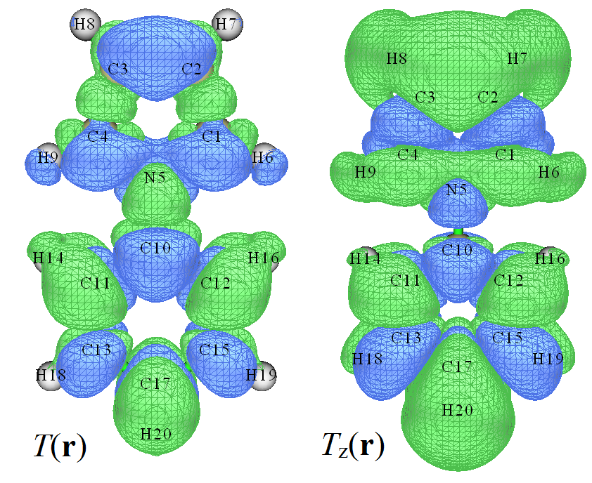
From the above T(r) map, we can see that hole and electron have strong coherence everywhere, implying that distribution of both hole and electron covers the whole molecule (this can be easily further confirmed by visualizing hole and electron distributions, as illustrated in Section 4.18.1). From the right map shown above one can see that its positive (green) part is obviously larger than negative (blue) part, recall that the integral of \(T_{\mathrm{z}}(\mathbf{r})\) over the whole space is just the Z component of transition electric dipole moment (\(D_{\mathrm{z}}\)), this observation explains why \(D_{\mathrm{z}}\) of S0→S1 is a large positive value (1.7813 a.u.). If you are interested, you can try to plot \(T_{\mathrm{x}}(\mathbf{r})\) or \(T_{\mathrm{y}}(\mathbf{r})\) maps to interpret why the electron excitation under study has vanished \(D_{\mathrm{x}}\) and \(D_{\mathrm{y}}\).
It is important to note that the S0→S1 of current system is relatively special, namely its transition electric dipole moment vector (D) just points towards Z-axis. However, for most practical cases, the D is not parallel to any of the three Cartesian axes, in this case we are not able to directly study its source in terms of visualization of any of \(T_{\mathrm{x}}(\mathbf{r})\) or \(T_{\mathrm{y}}(\mathbf{r})\) or \(T_{\mathrm{z}}(\mathbf{r})\). Fortunately, it is quite easy to reorient the molecule so that the D exactly points towards a selected Cartesian axis, thus making the above analysis feasible. See Appendix 2 of Section 4.A.7 on how to realize this.
Next, we check isosurface of \(T_{\mathrm{z}}(\mathbf{r})\) for S0→S4 excitation. We first return to menu of main function 18, then repeat above steps, finally you will see
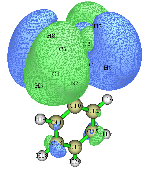
The green and blue isosurfaces occupy the same amount of space, indicating that positive and negative contributions to \(D_{\mathrm{z}}\) are exactly the same, this is why \(D_{\mathrm{z}}\) of S0→S4 is zero. Note that the \(T_{\mathrm{z}}(\mathbf{r})\) almost solely distributes on the pyrrole region, this is because this electron excitation corresponds to local excitation on pyrrole moiety (as shown in Section 4.18.1).
You may have felt that visual study of transition dipole moment density is interesting and useful; indeed, via this way you can clearly identify contribution to transition dipole moment from different molecular regions. The cube file of the T(r) as well as \(T_{\mathrm{x}}(\mathbf{r})\), \(T_{\mathrm{y}}(\mathbf{r})\) and \(T_{\mathrm{z}}(\mathbf{r})\) can be exported via post-processing menu, so that you can also plot them using other visualization software such as VMD (Section 4.A.14), or use such as basin analysis module (Section 3.20) or domain analysis module (Section 3.200.14) to further quantify their distributions, or plot them as plane map via main function 4 (using interpolated function based on loaded grid data, i.e. user-defined function -1).
Visualizing transition magnetic dipole moment density
The transition dipole moment we discussed above is transition electric dipole moment. There are also other kinds of transition dipole moments, such as transition velocity dipole moment and transition magnetic dipole moment. Multiwfn is also capable of calculating transition magnetic dipole moment and plotting the corresponding density isosurface map, related knowledge can be found in "Theory 5" of Section 3.21.1. Since this quantity is less important than transition electric dipole moment, I will not discuss it deeply, but only give a simple example. Using the .out and .fch files of N-phenylpyrrole, we first enter hole-electron module and select the second excited state, then input
-1 // By default, transition magnetic dipole moment density is not calculated by option 1 of hole-electron module for saving time, we select this option now to make option 1 also calculate this quantity
1 // Visualize and analyze hole, electron, transition density and so on
2 // Medium-quality grid
Once the calculation is finished, from screen you can find the transition magnetic dipole moment evaluated based on the grid data:
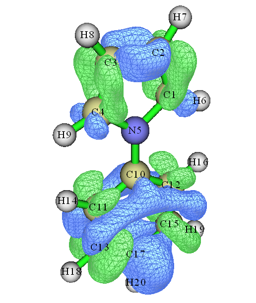
Then we select option 9 and select the component of transition magnetic dipole moment density that you are interested in, after that you will see the corresponding isosurface map. The following map is X component of transition magnetic dipole moment density plotted under isovalue of 0.005. The relatively larger blue region compared to green region explains why the X component of transition magnetic dipole moment is a negative value (-0.503 a.u.).
4.18.2.2 Plotting and analyzing transition density matrix (TDM)
Note
There is a video illustrating the procedure of using Multiwfn and Origin to plot the transition density matrix, see https://youtu.be/JPlZk4Aa6bQ.
The transition density matrix (TDM) has been carefully introduced in Section 3.21.2, heat map of TDM is particularly useful in understanding the nature of electron excitation, please read Section 3.21.2 first. In this section, we will analyze transition character of a linear system of donor-π-acceptor type by means of the TDM heat map. The molecular structure is shown below.
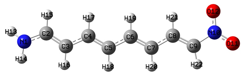
The Gaussian output file as well as .fchk file can be found in "examples\excit\NH2_C8_NO2" folder, the keyword is CAM-B3LYP/6-31G* IOp(9/40=4) TD(nstates=10).
It is worth to note that the TDM is closely related to the charge transfer matrix defined in hole-electron analysis framework. Example of plotting heat map of charge transfer matrix is given in Section 4.18.8.2. Usually heat maps of TDM and charge transfer matrix are very similar to each other and convey basically the same information.
Atom transition density matrix
First, we plot heat map of "atom TDM", namely the index of the TDM corresponds to atom index. Commonly, this kind of map is only suitable for studying chain-like systems such as the present molecule, otherwise the indices in the heat map will be difficult to be mapped to actual atoms in the molecule. For systems with more complicated shape, typically "fragment TDM" should be plotted instead, it will be described later.
Note that in "atom TDM", hydrogens are commonly ignored because they rarely contribute to excitations of chemical interest. Therefore, before the excited state calculation of the present molecule, the indices of the hydrogens have been moved to the back of heavy atoms. As can be seen from the molecular structure graph shown above, the range of heavy atoms is 1~12, while that of hydrogens is 13~22.
Here we first study S0→S1 transition of this system. The fchk and .out files used below are yielded using CAM-B3LYP/6-31G* IOp(9/40=4) TD(nstates=10) keywords. Boot up Multiwfn and input
examples\excit\NH2_C8_NO2\NH2_C8_NO2.fchk
18 // Electron excitation analysis
2 // Plot heat map of transition matrix
examples\excit\NH2_C8_NO2\NH2_C8_NO2.out
1 // Study transition between ground state to the 1st excited state. Then Multiwfn will calculate corresponding TDM
n // Do not diagonalize the newly generated TDM, because TDM in original form carries more useful information
1 // As mentioned in Section 3.21.2, there are several ways that can contract the TDM (represented in basis functions) to atom TDM. Here we use way 1. Way 2 and way 3 can also be used and can result in similar maps, while way 4 is usually deprecated
1 // Plot heat map
The map below is immediately shown on screen, the pink line was manually added to highlight the diagonal, the "hole" and "electron" texts were also manually labelled. By default, the lower limit of color scale is 0, while upper limit is the largest matrix element.
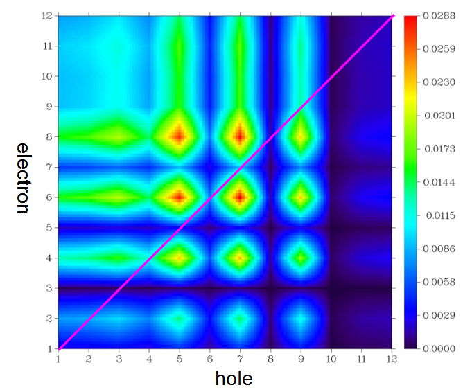
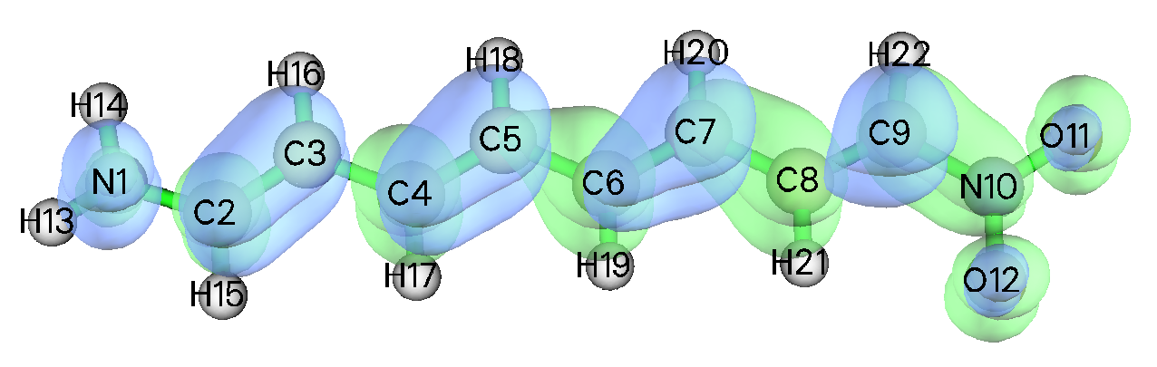
Electron excitation can be regarded as hole→electron transition. As introduced in Section 3.21.2, the diagonal terms of TDM heat map can reflect that in which atoms the hole and electron simultaneously have large distribution. For off-diagonal elements, we should first examine X-axis (corresponding to hole position) and then Y-axis (corresponding to electron position), we will be able to recognize how electrons transfer among different sites. In the TDM map of present instance, most elements in the diagonal are surrounded by green or red color, therefore this excitation must be a global excitation, namely the excited electrons distribute over the whole system. The matrix elements are not symmetric with respect to diagonal, it can be clearly seen that the upper left part of the map is larger than the lower right part, in particular, the elements near the diagonal have relatively large value. This observation reveals that electrons on non-hydrogen atoms are transferred to atoms adjacent to them, more specifically, electrons on the atoms with smaller index tend to transfer to atoms with larger index. Since the index of non-hydrogen atoms is ordered from the amino group to the nitro group, hence it can be inferred that this S0→S1 excitation causes the electrons to move integrally from the amino end to the nitro end.
If you find it difficult to understand above texts, you can compare the TDM map with below hole&electron isosurface map (see Section 4.18.1 on how to plot it). You can find the TDM heat map and the isosurface map convey similar information, and can confirm all of our conclusions drawn based on the TDM map.
If you want to plot TDM heat map for other excited state, you can exit the heat map plotting function, then re-enter this function and select the state to be studied. It is worth to note that if you choose option "4 Toggle if taking hydrogens into account" once to switch its status to "Yes" and then replot, you will see the map below
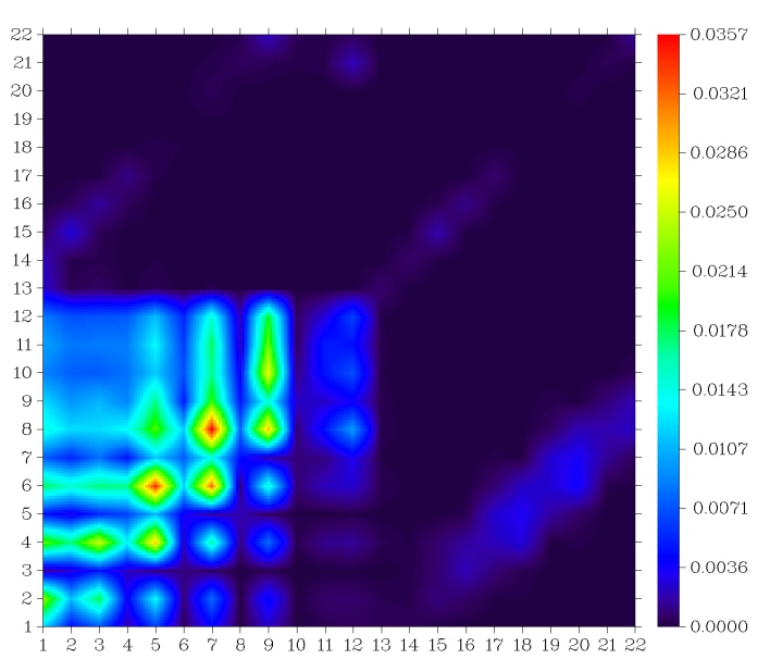
The index range of hydrogens are 13-22, the map above shows that hydrogens indeed do not evidently participlate in electron excitation because their elements are very small (represented as purple color), clearly it is meaningless to include hydrogens into S0→S1 TDM heat map.
Let us check another excitation, S0→S2. The heat map and hole&electron isosurface map are given below.
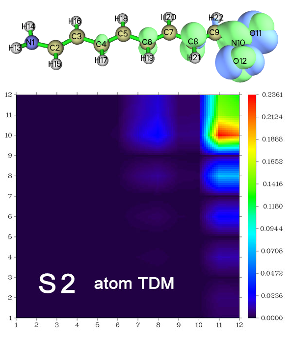
The upper right corner of the heat map has a large value area, which corresponds to the nitro group at the end of the system, therefore the hole and electron must have large distribution at the same time in this region. In addition, the value of the off-diagonal terms of rightmost column of the image is not very small, so it can be considered that the nitro group transfers a certain amount of electrons to the central region of the system, which is consistent with the phenomenon that can be seen in the hole&electron isosurface map. This observation can also be described as there is a so-called "coherence" between the nitro moiety and the intermediate region of the system in the S0→S2 excitation.
Fragment transition density matrix
Below we will plot TDM heat map based on fragment, namely the index of the map corresponds to the index of self-defined fragments. The advantage of this kind of TDM map is that the system to be studied is not necessarily linear, any shape of system (e.g. ring, star) can also be easily investigated.
The system to be investigated next is shown below, the molecule is divided into five fragments, which are represented as different colors. The Gaussian input, output and fchk files, as well as other files involved in the following texts can be downloaded from http://sobereva.com/attach/436/file.rar.
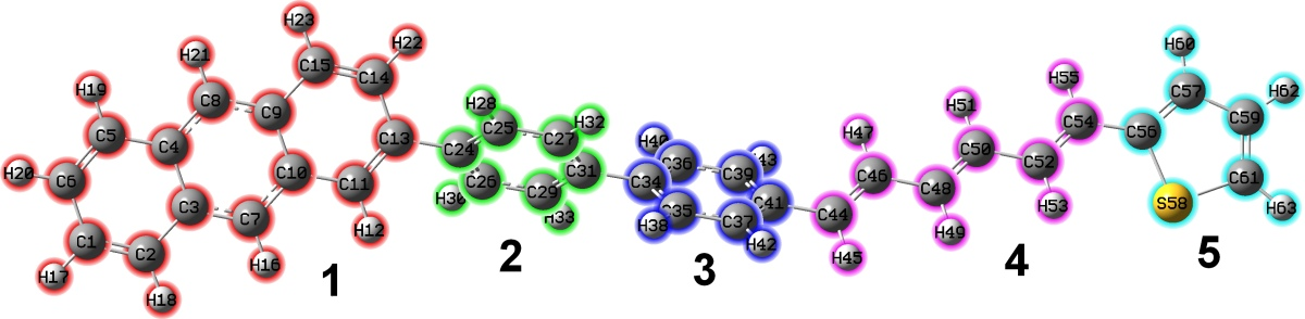
We first study S0→S1 excitation. Boot up Multiwfn and input
tdmat.fchk
18 // Electron excitation
2 // Plot heat map of transition matrix
tdmat.out
1 // Study S0→S1 excitation
n // Do not symmetrize the newly generated TDM
1 // Use the way 1 to contract the TDM represented in basis functions to atom TDM
Now you can choose option 1 to plot atom TDM. However, our present aim is to plot fragment TDM. In order to do this, we can create a plain text file (which has already been provided as tdmfrag.txt in the file.rar package), each line of it defines a fragment, the content of the file in this example is
Note that you can also use such as 2,5-8,12-15,20 to define a batch of atoms with discontinuous indices as a fragment.
Then input below commands
-1 // Define fragments
0 // Load fragment definition from an external file (as prompted, you can also directly input atom indices)
tdmfrag.txt // The file containing fragment definition
5 // Modify range of color scale
0,0.4 // Lower and upper limit
1 // Plot heat map
Now you can see the graph below, whose index corresponds to fragment index, the hole&electron isosurface map is also given together for comparison. The region marked with a blue frame is the 4th fragment (hexatriene).
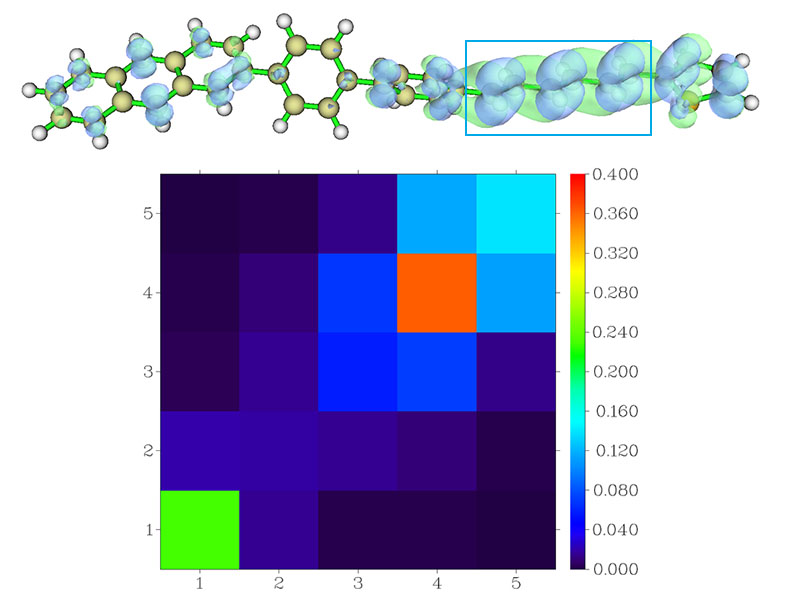
According to the colors in the heat map, we know that electron and hole are mainly distributed on fragment 4, but they also simultaneously appear on fragments 1 and 5 to some extent, these findings are consistent with the situation exhibited by the isosurface. Since no off-diagonal element in the graph is quite large, present electron excitation does not cause a significant electron transfer between various fragments. Roughly speaking, the main feature of this excitation is local excitation on fragment 4.
Analogously, we plot fragment TDM between ground state and each of S2~S7 excited states, the resulting maps are collectively shown below
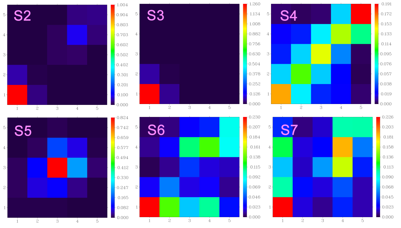
The values of the off-diagonal elements in the maps of S0→S2~S5 are not significant with respect to their diagonal elements, therefore interfragment electron transfer should not be obvious. According to the diagonal terms, we can find that the transitions of S0→S2 and S0→S3 mainly occurred in the fragment 1, while S0→S2 also marginally involves fragment 4. In general, both the transitions can be regarded as local excitation. The S0→S4 is evidently a global excitation since all diagonal terms are conspicuous. Main character of S0→S5 is local excitation on the fragment 3, which corresponds to a benzene ring, but its neighboring fragments are also more or less involved. S0→S6 and S0→S7 are somewhat mirrored with each other, from the figure it can be seen that almost every fragment is involved during electron excitation, they either occupied by hole distribution, electron distribution, or both. For S0→S6, we can speculate that the fragments 2, 3, and 4 transferred certain amount of electrons to the fragment 1 because (1,2), (1,3) and (1,4) elements are large, and meantime the fragments 3 and 5 also transferred some electrons to the fragment 4.
Above figure and discussion obviously show that, when you want to discuss transition character from ground state to a large number of excited states at the same time when writing an article, it is very straightforward to provide a figure containing TDM heat maps of all excitations.
Skill: Plotting TDM heat map for a batch of excited states using shell script
If you want to study a batch of excited states in terms of TDM heat map, while you feel that plotting maps one by one is laborious, you can use Linux shell script to fully automate this process.
The script that generates the fragment TDM heat maps for specified range of excited states at one time is examples\scripts\allTDM.sh. For example, if you put tdmat.fchk, tdmat.out, tdmfrag.txt, and allTDM.sh used in the example above into the Multiwfn directory and then enter this folder, run chmod +x allTDM.sh to add executable permissions, and then run ./allTDM.sh, this script will automatically call Multiwfn to generate 1.png, 2.png ... until 7.png in the current directory, they correspond to TDM heat map of S0→S1, S0→S2 ... to S0→S7. The entire process can be completed in a blink of an eye, clearly using the script is extremely convenient.
4.18.2.3 Plotting and analyzing transition dipole moment matrix
In fact, the heat map plotting function illustrated in last section is a general module, it can also plot other kinds of atom or fragment matrix. In Section 3.21.11, the concept of atom transition dipole moment matrix (atom TDMM) is introduced. This matrix has three components X, Y and Z. For example, the sum of all elements of the X component matrix just corresponds to the X component of transition dipole moment. Therefore, by plotting TDMM as heat map, we are able to make clear which atoms or fragments have conspicuous contributions to transition dipole moment.
Below, we still use the donor-π-acceptor employed in Section 4.18.2.2 as example to show how to plot TDMM as heat map. Multiwfn is able to plot both transition electric dipole moment matrix and transition magnetic dipole moment matrix, present section will limit to the former one.
Initially we need to generate a file containing atom TDMM. Boot up Multiwfn and input
examples\excit\NH2_C8_NO2\NH2_C8_NO2.fchk
18 // Electron excitation analysis
11 // Decompose transition dipole moment as basis function and atom contributions
examples\excit\NH2_C8_NO2\NH2_C8_NO2.out
1 // Study S0→S1 excitation
1 // The transition dipole moment to be studied is "electric"
y // Export atom TDMM
As shown in screen, matrices have been exported to .txt files in current folder with "AAtrdip" prefix, in which the AAtrdipX.txt contains the X component of atom TDMM. Next, we will plot heat map based on this matrix.
Reboot Multiwfn and input
o // Load the file last time loaded
18 // Electron excitation analysis
2 // Plot heat map of transition matrix
AAtrdipX.txt
Now you can find the information below on screen
 Sum of all elements (including hydrogens):     -4.38875223
 Maximum and minimum (including hydrogens):      0.65818572     -0.82543408
 Sum of all elements (without hydrogens):       -2.86353889
 Maximum and minimum (without hydrogens):        0.65818572     -0.82543408
where -4.38875223 is just the X component of transition electric dipole moment of S0→S1 excitation, the value is identical to that can be found from Gaussian output file.
As also shown in above prompt, the minimum value of this matrix is a negative value -0.825, however by default the lower limit of color scale of present function is 0, therefore we must change the color scale, and it is better to make absolute value of lower and upper limits identical. You can repeatedly try to find the value that makes the image best reflect the characteristics of the matrix. If the range is too narrow, the parts that exceed the upper and lower limits of the color scale will be displayed as white and black, respectively, which is not beautiful. If the range is too broad, the difference of the matrix elements can hardly be distinguished by colors.
Now we input below commands in Multiwfn
5 // Modify range of color scale
-0.7,0.7 // Lower and upper limits
1 // Plot heat map
Immediately you can see the graph below. In order to better understand the heat map, the isosurface of transition dipole moment density of X component is also shown together (see Section 4.18.2.1 on how to plot it)
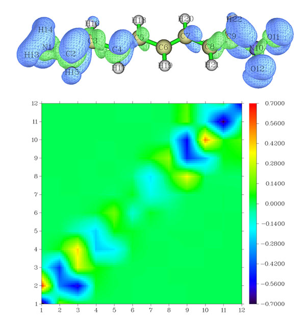
The bluer (redder) matrix element of this heat map contributes more negatively (positively) to the transition dipole moment of X component. Since most parts of the heat map are blue, the sum of all matrix elements must be negative, explaining why the X component of the transition dipole moment is a significant negative value (-4.388 a.u.). Because all matrix elements far from the diagonal are very close to 0 (shown as green), hence the long-range coupling between atoms does not contribute substantially to the transition dipole moment of X component. There are several areas of the figure show very blue color, such as the regions near (2,2) and (9,9), showing that corresponding atoms and neighboring ones have significant negative contributions, this point is also clearly reflected in the isosurface map of transition dipole moment density. Some sites such as (1,2) are obviously positive, which means that the coupling between the two atoms has a significant positive contribution to the transition dipole moment of X component, this is also why in the isosurface map there are green isosurfaces between atoms 1 and 2. The middle part of the heat map is basically green, indicating that the value is very small; correspondingly, there is no isosurface in the middle of the molecule on the isosurface map.
It can be seen that combining the transition dipole moment density and the transition dipole moment matrix together is helpful for clarifying the intrinsic characteristics of the transition dipole moment.
We can also plot TDMM based on fragment index, this is very easy and thus will not be further illustrated. What you need to do is simply defining fragments in the heat map plotting function and then plot the graph (please recall Section 4.18.2.3).
4.18.2.4 Investigating transition density and transition density matrix between excited states
In last several sections, I have illustrated how to study transition character in terms of transition (dipole moment) density as real space function and transition (dipole moment) density matrix between ground state and excited states. In fact, these kinds of studies can also be used to analyze transition between two excited states, such analyses may be useful in special applications, such as transient absorption spectrum and two-photon process. In this section, I will show how to realize these analyses.
Analysis of transition density in real space function between excited states
As shown in Section 4.18.2.1, Multiwfn is able to easily generate grid data of transition density between ground state and a selected excited state. In fact, transition density between two excited states can also be generated. To do so, we should first generate transition density matrix (TDM) between the two states, however, since all analyses related to real space function in Multiwfn are based on orbitals, we then need to transform the TDM to corresponding natural orbitals. Finally, the electron density evaluated based on these natural orbitals will directly correspond to transition density.
Here S2→S3 transition of N-phenylpyrrole is taken as an example, below procedure will generate cube file of corresponding transition density. Boot up Multiwfn and input
examples\excit\N-phenylpyrrole.fch
18 // Electron excitation analysis
9 // Generate and export transition density matrix
2 // Generate transition density matrix between (TDM) two excited states
examples\excit\N-phenylpyrrole.out
2,3 // Assume that you want to analyze S2→S3 transition
[Press ENTER button directly to use default threshold]
y // Symmetrize the resulting TDM in usual way
y // Export present wavefunction information including the newly generated TDM to TDM.fch in current folder
Reboot Multiwfn and input
TDM.fch
200 // Other function, part 2
16 // Generate natural orbitals based on the density matrix in .fch/.fchk file
SCF // We input this because the "Total SCF Density" field in the TDM.fch currently correspond to S2→S3 TDM
y // Export new.mwfn, which contains natural orbitals corresponding to S2→S3 TDM, and then let Multiwfn directly load it
0 // Return to main menu
5 // Calculate grid data
1 // Electron density
2 // Medium-quality grid
2 // Export cube file
Now the generated density.cub in current records transition density between S2 and S3, you can also choose option -1 to directly visualize the isosurface.
It is also possible to generate grid data of transition dipole moment density between excited states. For example, if you set “iuserfunc” parameter in settings.ini to 22, which sets user-defined function to \(-x\rho(\mathbf{r})\), then when you use the new.mwfn generated previously as input file, the user-defined function will correspond to X component of transition dipole moment density of S2→S3 transition. Clearly, what you should do next is calculating grid data of user-defined function.
Heat map of transition density matrix between excited states
Here we use the NH2-C8-NO2.fchk and NH2-C8-NO2.out employed in Section 4.18.2.2 as example to illustrate how to plot heat map of transition density matrix between two arbitrarily selected excited states, S1 and S2.
Boot up Multiwfn and input
examples\excit\NH2_C8_NO2\NH2_C8_NO2.fchk
18 // Electron excitation analysis
9 // Generate transition density matrix
2 // For two excited states
examples\excit\NH2_C8_NO2\NH2_C8_NO2.out
1,2 // The states are chosen as S1 and S2
[Press ENTER button to use default threshold]
0 // Do not symmetrize the resulting TDM
n // Do not yield TDM.fch
Now we have tdmat.txt in current folder, which records TDM of S1→S2.
Reboot Multiwfn and then input
o // Load the file last time loaded
18 // Electron excitation analysis
2 // Plot heat map for transition matrix
tdmat.txt // Matrix data will be loaded from this file
1 // Construct atom transition matrix in terms of way 1
1 // Plot heat map
The obtained graph is shown below, the isosurface map of density difference yielded by subtracting S1 density from S2 density is also given (see Section 4.18.13 on how to plot it).
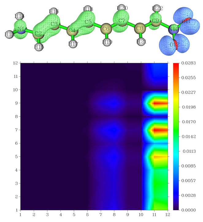
Since the area corresponding to atoms 1~9 at the right side (X=11 and 12) of the heat map has large value, we can speculate that a large amount of electrons is transferred from atoms 11 and 12 to atoms 1~9 during the S1→S2 excitation. Exactly same conclusion can also be gained from the isosurface map of density difference. This example shows that the density matrix heat map is not only useful and reliable for analyzing transitions from ground state to excited states, but also for transitions between various excited states.
4.18.3 Analyze charge-transfer during electron excitation based on electron density difference
Note
Blog article “Using Multiwfn to analyze charge transfer based on electron density difference descriptors” (in Chinese, http://sobereva.com/776) contains significantly more information than this section.
In this instance we will analyze charge-transfer (CT) between the first singlet excited state and ground state of the molecule shown below in ethanol solvent, which will be referred to as P2. The related theory has been introduced in Section 3.21.3. The discussions in this example are somewhat related to the ones involved in Section 4.18.1, however the method employed in this section is purely based on electron density difference, therefore it is more universal and can be used for any theoretical methods that can generate wavefunctions of ground state and excited state (e.g. CCSD in combination with EOM-CCSD).
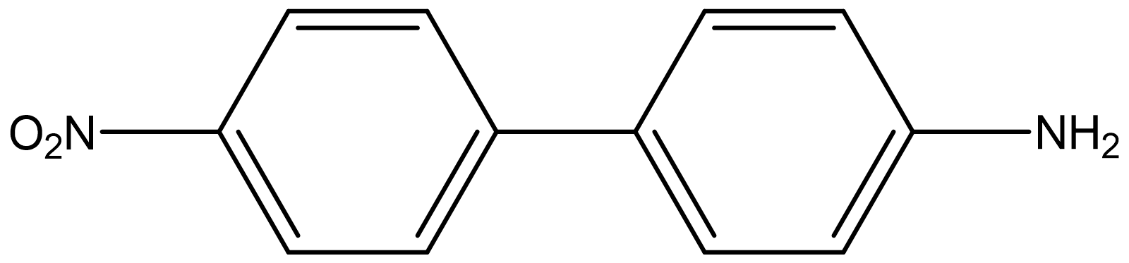
Since the .wfn files corresponding to the excited state and ground state are large, they are not provided. Instead, the input files of Gaussian for generating the two .wfn files are provided in “examples\excit” folder (extP2.gjf and basP2.gjf). I assume that the corresponding .wfn files are produced at "CT" subfolder in current folder. I would like to remind you once again, the geometries in the wavefunction files of the two states must be exactly identical, otherwise the result will be meaningless! If you do not have Gaussian in hand, you can also directly download the extP2.wfn and basP2.wfn from http://sobereva.com/multiwfn/extrafiles/extP2_basP2.zip.
First, we calculate grid data of electron density variation Δρ during the excitation. Boot up Multiwfn and input:
CT\extP2.wfn // Excited state wavefunction file
5 // Generate grid data
0 // Set custom operation
1 // Only one file will be dealt with
-,CT\basP2.wfn // Ground state wavefunction file. Corresponding density will be subtracted from the excited one to generate Δρ
1 // Electron density
2 // Medium-quality grid. If the system is much larger than present one, more grid points is required (e.g. using high-quality grid)
Once the calculation is normally completed, you can choose option -1 to view the electron density variation during the electron excitation (default isovalue is too large for visualizing density difference, 0.005 is recommended for present case). Green and blue regions correspond to positive and negative regions, respectively, they represent increase and decrease in electron density due to the excitation.
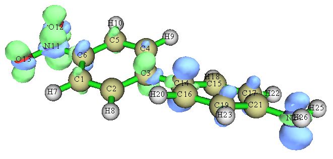
However this density difference graph is not quite intuitive, since positive and negative parts intertwined together and there are many nodes. We will see that \(C_+\) and \(C_-\) functions make the image much clearer.
0 // Return to main menu
18 // Electron excitation analysis
3 // Analyzing CT based on electron density difference grid data
The following information is displayed immediately. Note that if positive and negative parts of \(q_{\mathrm{CT}}\) are obviously unequal, that means the grid setting used in generating Δρ is too coarse, and you need to calculate again with finer grid setting.
 q_CT (positive and negative parts):   0.844  -0.844 a.u.
 Barycenter of positive part in x,y,z (Angstrom):  -2.659  -0.001  -0.000
 Barycenter of negative part in x,y,z (Angstrom):   2.294  -0.009  -0.029
 Distance of CT in x,y,z (Angstrom):   4.953   0.009   0.029  D index:   4.953
 Dipole moment variation (a.u.) :   7.896  -0.014  -0.046 Norm:   7.896
 Dipole moment variation (Debye):  20.070  -0.035  -0.117 Norm:  20.070
 RMSD of positive part in x,y,z (Angstrom):  2.993  1.250  0.821 Total:   3.346
 RMSD of negative part in x,y,z (Angstrom):  3.290  1.144  0.881 Total:   3.593
 Difference between RMSD of positive and negative parts (Angstrom):
 X:  -0.297  Y:   0.106  Z:  -0.060  delta_sigma index:  -0.247
 H_x:  3.141  H_y:  1.197  H_z:  0.851  H_CT:  3.141  H index:  3.469 Angstrom
 t index:   1.811 Angstrom
 Overlap integral between C+ and C- (i.e. S+- index):  0.742365
Above information is self-explanatory, if you are confused, please consult Section 3.21.3. The evident positive value of t index implies that the distribution of positive and negative of Δρ has been significantly separated due to strong CT. The large D index (4.95 Å) shows that the CT distance is quite long. Clearly, S0→S1 transition of this system should be identified as typical CT excitation. The excitation caused significant variation of dipole moment, as shown in the data, it is as high as 20.07 Debye. The distribution spatial distribution breadth of positive and negative parts of Δρ are similar, therefore the outputted Δσ index, which measures difference of their RMSD, is merely -0.247 Å.
By selecting option 1, isosurface of \(C_+\) (green) and \(C_-\) (blue) functions can be shown up. The isovalue of the graph shown below is 0.0015.
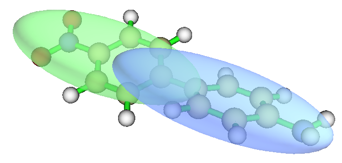
If the isovalue is increased to 0.0024, the positions of barycenters can be approximately located (barycenters of \(C_+\) and \(C_-\) exactly correspond to center of their isosurfaces).
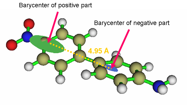
From the graph it is evident that the direction of electron transfer is from the amino group side (electron donor) to nitro group side (electron acceptor). However, the barycenters are not exactly located at the two substituents, this observation suggests that the actual electron donor in this electron excitation is not solely the amino group but also the phenylene. This finding parallels to the fact that phenyl is a weak electron donor.
Hint
If you would like to get better display effect of the C+ and C- isosurfaces, you can use VMD program (freely available at http://www.ks.uiuc.edu/Research/vmd/) to display them, the procedure is: Boot up VMD first, drag Cpos.cub into VMD main window, and then drag Cneg.cub into it. Select "Graphics"-"Representations", choose the first term in "Selected Molecule", click "Create Rep" button to create a new representation (the existing representation is used to show molecular structure), change the "drawing method" to "isosurface", set "Draw" to "solid surface", change the isovalue to 0.0015, set "coloring method" to "ColorID" and choose "7 green". Now the isosurface of Cpos has been properly displayed. Next, choose the second term in "Selected Molecule", use the similar methods to set each option, but select "0 blue" in "ColorID", and use isovalue of -0.0015. Finally, the graph will look like the one shown above. You can also set "Material" to "transparent" so that the overlap region of C+ and C- can be clearly distinguished.
4.18.4 Calculate ∆r and Λ indices to characterize various electron excitations for N-phenylpyrrole
In this section I will illustrate how to calculate the Δr index proposed in J. Chem. Theory Comput., 9, 3118 (2013) and the Λ index proposed in J. Chem. Phys., 128, 044118 (2008) to characterize electron excitations for N-phenylpyrrole. If you are not familiar with these two indices, please check Section 3.21.4 and Section 3.21.14, respectively.
In my personal view, using quantities such as D and \(S_{\mathrm{r}}\) indices defined in hole-electron framework to characterize electron excitation is already absolutely sufficient, as illustrated in Section 4.18.1. Theoretically, the Δr and Λ indices may be regarded as approximations of D and \(S_{\mathrm{r}}\), respectively. The only advantage of Δr and Λ is that in Multiwfn, they can be outputted for all selected excited states at the same time and can be decomposed into orbital pair contributions. In addition, calculation cost of Δr index is almost negligible.
The files used in this section are N-phenylpyrrole.fch and N-phenylpyrrole.out in "examples\excit" folder, they were yielded by Gaussian, the keywords are CAM-B3LYP/6-31+G(d) TD(nstates=5) IOp(9/40=4). Since the optimized ground state geometry was used in the calculation, therefore the analysis results can be regarded as corresponding to vertical absorption process.
Calculating Δr index
The Δr index is a quantitative indicator for measuring charge transfer (CT) length of electron excitation, larger Δr index implies longer CT distance.
Boot up Multiwfn and input
examples\excit\N-phenylpyrrole.fch
18 // Electron excitation analysis
4 // Calculate Δr index
examples\excit\N-phenylpyrrole.out
1-5 // Assume that we want to calculate Δr index for all the five calculated singlet excited states
Immediately, the results are printed on screen:
 Excited state    1:   Delta_r =    1.499249 Bohr,    0.793368 Angstrom
 Excited state    2:   Delta_r =    3.489064 Bohr,    1.846333 Angstrom
 Excited state    3:   Delta_r =    4.641132 Bohr,    2.455982 Angstrom
 Excited state    4:   Delta_r =    5.869424 Bohr,    3.105966 Angstrom
 Excited state    5:   Delta_r =    7.091127 Bohr,    3.752463 Angstrom
The Δr indices imply that the excitations from ground state (S0) to the 3th, 4th and 5th excited states possess strong CT character since they have large Δr, while the excitations of S0→S1 and S0→S2 should be basically regarded as LE excitations because their Δr indices are not quite large (the original paper of Δr suggests using 2.0 Å as criterion for distinguishing LE and CT excitations). Bear in mind, definitive conclusion about the excitation character can only be finally drawn after visualizing the hole and electron distributions using the hole-electron analysis module of Multiwfn.
In Multiwfn it is possible to decompose the Δr index as contributions of orbital pair transitions. For example, we want to do this for the S0→S4 excitation, we should first enter the Δr index calculation interface and then input
4 // Only calculate Δr index for a single excitation (S0→S4), in this case the result can be decomposed
y // Print orbital pair contributions
0.01 // Only the orbital pairs having contribution larger than 0.01 Å will be printed
You will immediately see the information below
Note: The configuration coefficients shown below have combined both excitation
and de-excitation parts
 Sum of square of configuration coefficients:    0.497953
    #Pair     Orbitals      Coefficient     Contribution (Bohr and Angstrom)
     378     37     41       0.5004500          3.7301590       1.9739153
     379     37     43       0.4452400          1.8477898       0.9778083
     381     37     47      -0.1067900          0.0929645       0.0491947
     382     37     49      -0.0782100          0.0700060       0.0370456
     383     37     53      -0.0639300          0.0285116       0.0150877
     389     37     72       0.0436900          0.0215865       0.0114231
As you can see, MO37→MO41 transition has predominating contribution (1.97 Å) to the Δr index of S0→S4 (3.11 Å), while the MO37→MO43 transition also has nonnegligible contribution (0.97 Å).
Calculating Λ (lambda) index
The Λ index essentially measures overlapping degree of hole and electron of electron excitations. Here we calculate it for all the five excitations for N-phenylpyrrole.
Boot up Multiwfn and input
examples\excit\N-phenylpyrrole.fch
18 // Electron excitation analysis
14 // Calculate Λ index
examples\excit\N-phenylpyrrole.out
1-5 // Analyze all the five calculated singlet excited states
Immediately, the results are printed on screen:
 Excited state    1:   lambda =    0.684853
 Excited state    2:   lambda =    0.563804
 Excited state    3:   lambda =    0.530928
 Excited state    4:   lambda =    0.198710
 Excited state    5:   lambda =    0.235255
From above output, it can be found that the Λ indices are nearly inversely proportional to the Δr indices, because the larger the hole-electron overlapping extent, usually the shorter the hole-electron separation distance (but bear in mind, this relationship is not always true).
Then we decompose the Λ index for the fourth excitation. Input below commands
y // Do the Λ index analysis again
4 // The fourth excitation
y // Decompose analysis on Λ index
0.01 // Printing threshold
Then you will see all MO pairs having contribution to Λ index larger than 0.01:
Sum of square of configuration coefficients:    0.497953
    #Pair     Orbitals      Coefficient     Contribution
     378     37     41       0.5004500          0.0865190
     379     37     43       0.4452400          0.0915297
The data indicates that only occupied MO 37 has a non-negligible overlap with unoccupied MOs; specifically, only the overlap between MO37-MO41 and between MO37-MO43 is relatively detectable.
4.18.5 Calculate dipole moment of each excited state and transition dipole moment between all states for 4-nitroaniline
This example will utilize the function described in Section 3.21.5, please read it first to gain relevant knowledge. In this example I use 4-nitroaniline to illustrate how to calculate electric dipole moment of each state, and then illustrate how to calculate transition magnetic dipole moment between all states. The state in this context refers to ground state and excited states obtained by TDDFT calculation. The corresponding Gaussian TDDFT input file for generating the .fch and .out files used in this example is examples\excit\4-nitroaniline.gjf.
Boot up Multiwfn and input
examples\excit\4-nitroaniline.fch
18 // Electron excitation analysis
5 // Calculate transition electric/magnetic dipole moments between all states and for each state
examples\excit\4-nitroaniline.out
4 // Obtain electric dipole moment of each state
Now you have dipmom.txt in current folder, you can see electric dipole moments of ground state and various excited states.
 Note: The electric dipole moments shown below include both nuclear charge and electronic contributions
 Ground state electric dipole moment in X,Y,Z:    0.326322   -2.792165    0.000000 a.u.

 Excited state electric dipole moments (a.u.):
  State         X             Y             Z        exc.(eV)    exc.(nm)
     1      0.334929     -1.219854      0.000000      4.0557      305.70
     2      0.251666     -7.797482      0.000000      4.2762      289.94
     3      0.334065     -1.439663      0.000000      4.5846      270.44
Next, we calculate transition magnetic dipole moment between all states. Boot up Multiwfn and input
examples\excit\4-nitroaniline.fch
18 // Electron excitation analysis
5 // Calculate transition electric/magnetic dipole moments between all states and for each state
examples\excit\4-nitroaniline.out
0 // Choose type of (transition) dipole moment to be calculated
2 // Magnetic
1 // Output (transition) dipole moments on screen
Now you can see
Transition magnetic dipole moment between ground state (0) and excited states (
a.u.)
     i     j         X             Y             Z        Diff.(eV)
     0     1    -0.0005545    -0.6041898    -0.0000000     4.05570
     0     2     0.0000000    -0.0000000     0.0137951     4.27620
     0     3     0.0000000    -0.0000000     1.0423466     4.58460

 Transition magnetic dipole moment between excited states (a.u.):
     i     j         X             Y             Z        Diff.(eV)
     1     1    -0.0000000    -0.0000000    -0.0113149     0.00000
     1     2     0.0060715     0.1120542     0.0000000     0.22050
     1     3    -0.2144702     0.0000589     0.0000000     0.52890
     2     2    -0.0000000    -0.0000000    -0.0099328     0.00000
     2     3    -0.0000000    -0.0000000    -0.1215811     0.30840
     3     3    -0.0000000    -0.0000000    -0.0074159     0.00000
From above output you can find transition magnetic dipole moment between ground state and excited states, as well as between various excited states.
Similarly, you can calculate transition electric dipole moment between various states.
4.18.6 Generate and analyze natural transition orbitals (NTOs) for uracil
Note
Chinese version of this section is my blog article “Using Multiwfn to perform natural transition orbital (NTO) analysis” (http://sobereva.com/377), which contains extended discussions.
In this section I illustrate how to use Multiwfn to perform the very popular natural transition orbital (NTO) analysis with uracil as example. Please first read Section 3.21.6 to acquire basic knowledge of NTO. Although in this example the files outputted by Gaussian were used as input file, in fact the files outputted by ORCA are also fully supported, see Section 3.21.1.2 for detailed requirements about the input file.
Before showing how to perform NTO analysis, I would like to let you apprehend why NTO analysis is meaningful. As an instance, we use Gaussian to perform TDDFT calculation at PBE0/6-31G* level for singlet excited states of uracil, you will find the following information
Excited State   3:      Singlet-A"     6.0180 eV  206.02 nm  f=0.0000  <S**2>=0.000
      26 -> 30         0.54135
      26 -> 31        -0.20634
      28 -> 30        -0.15424
      28 -> 31         0.36715
Clearly, in excitation of S0→S3, there is no dominant MO transition, the largest contribution of a single MO pair is merely 0.541^2*2*100%=58.5%, therefore it is impossible to identify the nature of this excitation by viewing only one MO pair. In such difficult cases, NTO analysis is often useful, because after transforming MOs into NTOs, commonly you will be able to find only one pair of NTO having eigenvalue very close to 1, transition between the two NTOs in this pair faithfully represents the real character of the electron excitation.
The files needed by NTO analysis have been mentioned at the beginning of Section 3.21. Briefly, assume that you are a Gaussian user and you want to study electron excitation from ground state to the lowest three singlet excited states for uracil at TD-PBE0/6-31G* level, what you need to do is carrying out a normal TDDFT calculation with these keywords: # PBE1PBE/6-31G* TD IOp(9/40=4), also you need to make Gaussian generate corresponding .fch file. The input file, output file and .fch file have already been provided in "examples\excit\NTO" folder. The keyword IOp(9/40=4) is very important, without it the NTO result will be evidently inaccurate, the meaning of this IOp has been mentioned in Section 4.18.1.
Now we start to carry out NTO analysis. Boot up Multiwfn and input
examples\excit\NTO\uracil.fch
18 // Electron excitation analysis
6 // Generate NTOs
examples\excit\NTO\uracil.out // Gaussian calculated three lowest excited states, you can analyze any one of them
3 // Study transition from ground state (S0) to the 3rd excited state (S3)
Now Multiwfn loads transition information of S0→S3 from the Gaussian output file and generate NTOs, the eigenvalues of NTO pairs are shown below
The highest 10 eigenvalues of NTO pairs:
   0.865529    0.134025    0.000582    0.000121    0.000063
   0.000024    0.000016    0.000015    0.000007    0.000006
Sum of all eigenvalues:  1.000387
It can be seen that the largest eigenvalue is 0.8655, that means that NTO pair contributes as high as 86.55% of the S0→S3 transition. So, if we would like to characterize the nature of this transition, we can only study the occupied NTO and virtual NTO in this NTO pair.
Now you can select if outputting .fch/.mwfn/.molden file containing the NTOs. We choose "3 Output NTO orbitals to .mwfn file" and input the path to output, such as C:\S3.mwfn. After the .mwfn has been successfully generated, you can reboot Multiwfn and load the S3.mwfn, in main function 0 you can visualize the NTOs, the orbital energies now correspond to NTO eigenvalues. To plot the occupied and virtual NTOs corresponding to the NTO pair with 86.55% contribution, in the GUI of main function 0 you can select "orbital info." - "Show up to LUMO+10" in the menu, in the text window you will find output like below
Orb:    27 Ene(au/eV):     0.000582       0.0158 Occ: 2.000000 Type: A+B
Orb:    28 Ene(au/eV):     0.134025       3.6470 Occ: 2.000000 Type: A+B
Orb:    29 Ene(au/eV):     0.865529      23.5522 Occ: 2.000000 Type: A+B
Orb:    30 Ene(au/eV):     0.865529      23.5522 Occ: 0.000000 Type: A+B
Orb:    31 Ene(au/eV):     0.134025       3.6470 Occ: 0.000000 Type: A+B
Orb:    32 Ene(au/eV):     0.000582       0.0158 Occ: 0.000000 Type: A+B
We can see that the occupied NTO with index of 29 and the virtual NTO with index of 30 constitute the NTO pair with eigenvalue of 0.8655, there we select corresponding index in the GUI to visualize them, the isosurfaces are shown below
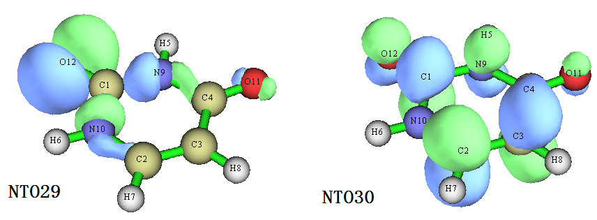
Undoubtedly, this S0→S3 excitation can be regarded as transition from lone pair of O12 to anti-bonding π orbital of the uracil ring, at least we have 86.55% confidence to say that. From NTO eigenvalues we notice that NTO28→NTO31 transition also has small contribution (13.40%) to the excitation, please plot corresponding orbitals and discuss their characteristic.
The NTOs can also be subjected to quantitative analyses. For example, you can enter main function 8 and use suitable options to analyze their orbital composition at quantitative level, or you can use subfunction 11 of main function 100 to evaluate overlap extent and centroid distance between selected two NTOs.
In Multiwfn it is possible to evaluate energies of orbitals in any kind. In Section 4.300.6 a detailed example of calculating energies of NTO orbitals is given.
It is worth to note that NTO analysis has both advantages and disadvantages with respect to the hole-electron analysis, this point has been mentioned at the end of Section 3.21.6. For many systems and excitations, even if NTO transformation has been applied, there are still no NTO pair with predominant contribution, in this case you have to resort to hole-electron analysis to facilitate discussion of excitation characteristic. The drawback of hole-electron analysis is that it is unable to present orbital phase information like NTO analysis, and it takes higher computational cost.
Using script to carry out NTO analysis in batch
Sometimes we want to perform NTO analysis for a batch of excitations, for example, we want to generate a batch of .fch files that respectively contain NTOs of S0→S1, S0→S2 and S0→S3 transitions, although you can manually do this in the interactive interface of Multiwfn, a more efficient and cleverer way is employing shell script. If you are a Linux user, we can run below shell script to yield S1.fch, S2.fch and S3.fch, which contain NTOs corresponding to S0→S1, S0→S3 and S0→S3. This script is very easy to understand as long as if you have basic level of knowledge about shell programming.
#!/bin/bash
cat << EOF > allNTO.txt
18
6
examples/NTO/uracil.out
EOF
for ((i=1;i<=3;i=i+1))
do
cat << EOF >> allNTO.txt
$i
2
S$i.fch
6
EOF
done
./Multiwfn examples/excit/NTO/uracil.fch < allNTO.txt
rm ./allNTO.txt
This script is also provided as examples\excit\NTO\allNTO.sh. If you do not make any modification to the script, this script should be copied to the Multiwfn folder and run as ./allNTO.sh in Multiwfn folder, then S1.fch, S2.fch and S3.fch will be yielded at the same folder. In practical studies, you should properly modify the script according to actual situation, the range of the excitations to be studied is determined by "i=1;i<=3".
4.18.8 Using IFCT method and heat map of charge transfer matrix to study interfragment charge transfer during electron excitation
The interfragment charge transfer (IFCT) is a method derived based on hole-electron analysis for quantitatively studying amount of charge transfer between different fragments. The situation of charge transfer can also be very intuitively understood by means of heat map of charge transfer matrix, which is a byproduct of IFCT analysis. Please carefully read Section 3.21.8 if you are not familiar with these concepts.
In the next two sections, I will use two molecules to respectively illustrate how to perform IFCT analysis and plot heat map of charge transfer matrix, these two kinds of analyses can provide complementary perspectives.
4.18.8.1 IFCT analysis for 4-nitroaniline
In this example, I will illustrate how to use IFCT method to study CT between three fragments (-NO2, -NH2 and the linker benzene) of 4-nitroaniline during its electron excitation.
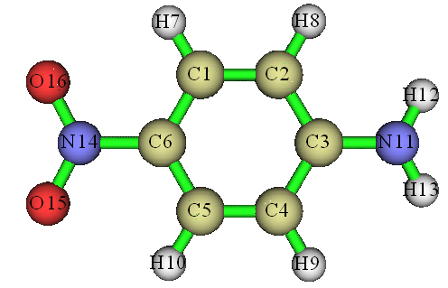
The Gaussian input file of TDDFT task at PBE0/6-311G* level for 4-nitroaniline has been provided as examples\excit\4-nitroaniline.gjf. Note that IOp(9/40=4) is used so that Gaussian can print enough configuration coefficients. Run it by Gaussian to obtain .chk file and .out file, then convert the .chk file to .fch via formchk. The .fch and .out files have been provided in "examples\excit" folder.
Boot up Multiwfn and input below commands
examples\excit\4-nitroaniline.fch
18 // Electron excitation analysis
8 // Calculate interfragment charge transfer in electron excitation via IFCT method
1 // Mulliken partition
[Press ENTER button] // Load examples\excit\4-nitroaniline.out
2 // We first analyze transition from ground state (S0) to the second excited state (S2)
3 // Define three fragments
11-13 // Atomic indices of amino group (fragment 1)
1-10 // Atomic indices of benzene group (fragment 2)
14-16 // Atomic indices of nitro group (fragment 3)
Then you will see
 Contribution of each fragment to hole and electron:
  1  Hole:  28.17 %     Electron:   3.02 %
  2  Hole:  65.89 %     Electron:  29.52 %
  3  Hole:   5.94 %     Electron:  67.46 %
 Construction of interfragment charger-transfer matrix has finished!

 Variation of population number of fragment  1:  -0.25150
 Variation of population number of fragment  2:  -0.36369
 Variation of population number of fragment  3:   0.61519

 Intrafragment electron redistribution of fragment  1:   0.00849
 Intrafragment electron redistribution of fragment  2:   0.19453
 Intrafragment electron redistribution of fragment  3:   0.04009

 Transferred electrons between fragments:
  1 ->  2:   0.08315       1 <-  2:   0.01987     Net  1 ->  2:   0.06328
  1 ->  3:   0.19001       1 <-  3:   0.00179     Net  1 ->  3:   0.18821
  2 ->  3:   0.44452       2 <-  3:   0.01754     Net  2 ->  3:   0.42697

 Intrinsic charge transfer percentage, CT(%):     75.688 %
 Intrinsic local excitation percentage, LE(%):    24.312 %
The output is very easy to understand, if you are confused, please check corresponding explanation in Section 3.21.8. For example, the data shows that during the S0→S2 excitation, nitro group (fragment 3) donates 0.00179 electrons to amino group (fragment 1) and meantime accept 0.19001 electrons from amino group, therefore nitro group totally gains 0.18821 electron from amino group. If the benzene fragment is also taken into account, the electron excitation totally increases electron population of nitro group by 0.61519. The electron redistribution phenomenon in the two terminal groups is not prominent, however, as the data shown (0.19453), the electron redistribution within the benzene, which behaves as π linker, is remarkable. Because CT(%) is notably larger than LE(%), this excitation can be mostly regarded as a charge transfer state.
For facilitating discussion, I summarized all IFCT analysis data in the table below. The diagonal terms correspond to amount of intrafragment electron redistribution.
| Donor | Amino group | benzene | nitro group |
|---|---|---|---|
| amino group | 0.008 | 0.083 | 0.190 |
| benzene | 0.020 | 0.195 | 0.445 |
| nitro group | 0.002 | 0.018 | 0.040 |
As you can see from the table, there are three prominent interfragment CT terms (sorted according to magnitude): benzene→nitro, amino→nitro, amino→benzene, all of them direct from amino group towards nitro group.
For better and intuitively understanding above data, we plot hole-electron isosurface map using the method described in Section 4.18.1:
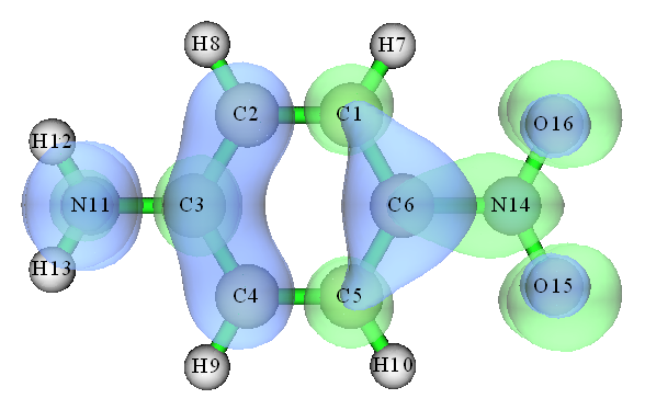
In the graph, main distribution regions of hole and electron correspond to blue and green, respectively. As you can see, hole mainly distributes on the amino group and benzene moiety, while electron mainly locates at the benzene linker and nitro group, clearly the overall CT direction is from amino group to nitro group, this is completely in line with our observation of quantitative interfragment CT analysis.
Using Hirshfeld partition
Commonly, the Mulliken-like partition, as what we have employed in this example, is a good choice because its calculation is quite fast and the result is usually reasonable. Unfortunately, it is incompatible with diffuse functions, and sometimes there are unphysical negative fragment contributions to hole or electron. When diffuse functions must be adopted (e.g. anionic system), or Multiwfn warns you that there are negative contributions, you should use the more robust Hirshfeld partition instead. It works well for any case, but the cost is markedly higher. To change to the Hirshfeld partition, you simply need to input 2 when Multiwfn asks you to select the method for calculating hole and electron composition. The data in the example above calculated by Hirshfeld partition is shown below; as you can see, the result is approximately identical to the result under Mulliken-like partition.
Intrafragment electron redistribution of fragment  1:   0.01047
Intrafragment electron redistribution of fragment  2:   0.19579
Intrafragment electron redistribution of fragment  3:   0.05327

Transferred electrons between fragments:
 1 ->  2:   0.08246       1 <-  2:   0.02485     Net  1 ->  2:   0.05761
 1 ->  3:   0.17946       1 <-  3:   0.00311     Net  1 ->  3:   0.17636
 2 ->  3:   0.42612       2 <-  3:   0.02448     Net  2 ->  3:   0.40164

Charge transfer percentage, CT(%):     74.047 %
Local excitation percentage, LE(%):    25.953 %
It is worth to notice that Multiwfn is able to calculate IFCT for a batch of excited states at once, hence can easily recognize major character of all excited states, see Section 4.18.6 for illustration.
More discussions and illustrations about the IFCT analysis can be found from my blog article "Using the IFCT method in Multiwfn to evaluate amount of electron transfer between arbitrarily defined two fragments during electron excitation" (in Chinese, http://sobereva.com/433).
4.18.8.2 Plotting heat map of charge transfer matrix to intuitively understand nature of electron excitation
The charge transfer matrix (CTM) is closely related to transition density matrix (TDM) and their heat maps often provide similar information for an electron excitation. The method of plotting TDM has been illustrated in Section 4.18.2.2. In my opinion, the physical meaning of CTM is somewhat clearer than TDM and can better reveal actual charge transfer character. In addition, since CTM is derived in the theory framework of hole-electron analysis (see Section 3.21.1), the CTM heat map can always well compare with distribution of hole and electron.
Here I still use the molecule studied in Section 4.18.2.2 as instance. Before plotting the heat map of CTM, we should first generate CTM. Boot up Multiwfn and input
examples\excit\NH2_C8_NO2\NH2_C8_NO2.fchk
18 // Electron excitation analysis
8 // IFCT analysis
1 // Mulliken-like partition to derive atomic contribution to hole and electron
examples\excit\NH2_C8_NO2\NH2_C8_NO2.out
1 // Study S0→S1 excitation
-1 // Export atom-atom CTM to atmCTmat.txt in current folder
2 // Enter the function used for plotting heat map
atmCTmat.txt // Load matrix data from this file
1 // Show heat map
Now you can see the map below, the purple line and texts are manually added.
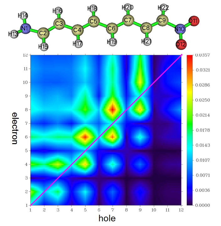
This figure has similar features of the heat map of atom TDM given in Section 4.18.2.2, but there are also differences that cannot be ignored. According to the IFCT point of view, each of the non-diagonal elements of the current graph rigorously exhibits the amount of electron transferred between atoms. Looking at the graph column by column, it can be visually seen that each atom on the carbon chain transferred electrons to the atoms at its front and back ends, and the amount of transfer to the nitro side is significantly more than to the amino side. For example, it can be seen from the figure that in the fifth column, the value of the sixth element is larger than the fourth element, so the amount of electron transfer of C5→C6 must be more than C5→C4.
Next, we also look into heat map of CTM of another excitation. The map of S0→S9 plotted in the same way as above is given below, corresponding hole&electron isosurface map is also appended. Because it was found that S0→S9 transition evidently involves some hydrogens, therefore hydrogens are also taken into account in the map (by choosing "4 Toggle if taking hydrogens into account" once).
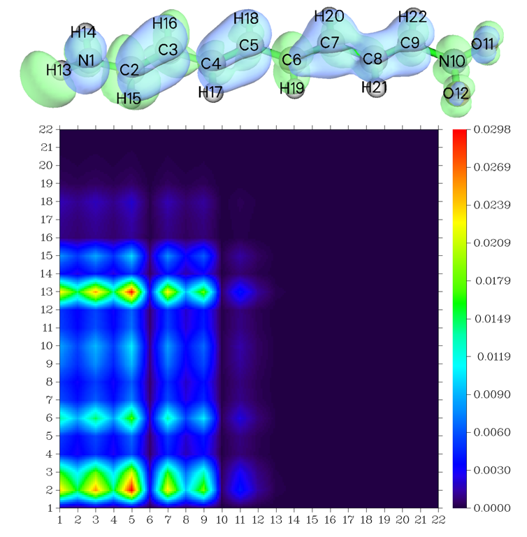
It can be seen from the above heat map that, there is strong electron transfer from the region of atoms 1~5 and 7~9 to the hydrogen atom with index of 13, this observation fully agrees with the hole&electron isosurface map, namely there is a large green isosurface at H13. In addition, from the isosurface map we can see that atom 6 is basically only surrounded by green isosurface, that means this atom does not transfer electrons to others while largely accepts electrons from others; accordingly, the color of the row of Y=6 in the heat map is distinct, while the column corresponding to X=6 is very dark.
From this example, we can find that the hole&electron isosurface map provides the most intuitive visual effect, but if it is discussed together with the heat map of CTM, the charge transfer can be understood more thoroughly from a quantitative point of view, it also avoids the possibility that the arbitrariness of the choice of isovalue leads to an unreasonable judgment.
The CTM can also be plotted based on fragment. To do this, you simply need to load fragment definition file or directly input fragment definition in the heat map plotting function, and then plot the map again.
4.18.9 Generate transition density matrix and transform it to orbital representation
Note
This section may not be interesting for most Multiwfn users, but valuable for experts
In Section 4.18.2, I have shown that in Multiwfn the transition density can be studied in terms of real space function and colored matrix (heat map). Multiwfn can do even more for transition density. As will be illustrated in this section, Multiwfn is able to transform the generated transition density matrix to orbital representation and export the orbitals as wavefunction file. This brings a lot of conveniences; for example, when you analyze "electron density" based on this file, the actual function to be studied will directly correspond to transition density. Note that these orbitals can be regarded as natural orbitals of transition density matrix (TDM), but they are remarkably different to the NTO (nature transition orbital), which has been introduced in Section 3.21.6.
Here will take the N-phenylpyrrole as example, whose transition density of S0→S1 has been plotted as isosurface in Section 4.18.2. Our purpose in this section is to transform this transition density into orbitals and export them as .wfx file so that then we can very easily study properties of the transition density based on this file.
First, we generate a .fch file containing TDM. Boot up Multiwfn and input
examples\excit\N-phenylpyrrole.fch // The .fch file yielded by Gaussian TDDFT task
18 // Electron excitation analysis
9 // Generate and export TDM
1 // Generate TDM between ground state and excited state
examples\excit\N-phenylpyrrole.out // The output file of Gaussian TDDFT task with IOp(9/40=4) keyword
1 // Analyze electron transition from ground state to the 1st excited state (S0→S1)
1 // Symmetrize the raw TDM. This is important, the natural orbitals cannot be properly yielded later without symmetrization of the TDM
y // Export current wavefunction to TDM.fch in current folder, whose "Total SCF Density" field records the just generated symmetrized TDM
Next, we transform the TDM into natural orbitals. Reboot Multiwfn and input
TDM.fch
200 // Other functions (Part 2)
16 // Generate natural orbitals based on the density matrix in .fch/.fchk file
SCF // The matrix to be transformed comes from the "Total SCF Density" field
y // Export the generated orbitals to new.mwfn and load it
Now we have new.mwfn in current folder, which contains natural orbitals transformed from the S0→S1 TDM. The orbitals in memory now also correspond to these natural orbitals. Assume that we also want to export them as .wfx file, we should input the commands below.
0 // Return to main menu
100 // Other functions (Part 1)
2 // Export various kinds of files
4 // Output current wavefunction as .wfx file
TDM.wfx // The path of the file to be generated
In the future, if you use the TDM.wfx as input file and calculate grid data of "electron density" via main function 5, you will find the resulting isosurface map (after properly adjusting isovalue) is exactly identical to the transition density T(r) graph shown in Section 4.18.2.1.
4.18.10 Obtain molecular orbital pair contributions to transition dipole moment
In order to gain a deeper insight into transition electric or magnetic dipole moment, Multiwfn provides a function used to decompose it to contributions from various MO pair transitions, see Section 3.21.10 for introduction. Here I present an example. The .fch and .out files involved in this example were produced by TDDFT calculation of Gaussian.
Boot up Multiwfn and input
examples\excit\N-phenylpyrrole.fch
18 // Electron excitation analysis
10 // Decompose transition dipole moment as molecular orbital pair contributions
1 // The type of transition dipole moment is electric
examples\excit\N-phenylpyrrole.out
1 // Select the excitation from ground state (S0) to the first singlet excited state (S1)
Now the information below about this excitation is shown on screen
 Transition dipole moment in X/Y/Z:   -0.000000  -0.000000   1.781438 a.u.
 Norm of transition dipole moment:     1.781438 a.u.
 Oscillator strength:   0.3935306
Then you can find several options on screen, they are self-explanatory. We first choose option 1 and input for example 0.02, then all MO pairs having contribution larger than 0.02 are printed:
#Pair   Orbital trans. Coefficient      Transition dipole X/Y/Z   Norm (a.u.)
  1213     35 ->     46   0.040230   0.000000   0.000000   0.037709   0.037709
  1214     35 ->     50  -0.047670   0.000000  -0.000000   0.040152   0.040152
  1239     36 ->     40  -0.101270   0.000000  -0.000000  -0.280355   0.280355
  1259     37 ->     40  -0.127550   0.000000   0.000000  -0.148489   0.148489
  1260     37 ->     52   0.069960  -0.000000  -0.000000  -0.122222   0.122222
  1262     37 ->     58  -0.036060  -0.000000   0.000000  -0.025065   0.025065
  1278     38 ->     39   0.672690  -0.000000   0.000000   2.796678   2.796678
  1280     38 ->     50   0.052570  -0.000000   0.000000   0.046724   0.046724
  2489     36 <-     40  -0.014330   0.000000  -0.000000  -0.039671   0.039671
  2506     37 <-     52   0.015140  -0.000000  -0.000000  -0.026450   0.026450
  2522     38 <-     39  -0.027240   0.000000  -0.000000  -0.113249   0.113249
Sum of the above      11 pairs:     -0.000000  -0.000000   2.165763
From the output, we can immediately find that transition of MO38→MO39 has dominating contribution (2.796678 a.u.) to this S0→S1 excitation.
When there are too many MO pairs having nonnegligible contributions to transition dipole moment and thus difficult to identify important MO transitions, you can let Multiwfn sort the MO pairs according to their contributions to specific component of transition dipole moment. For example, here we choose the option " 4 Print orbital pairs in the order of absolute contribution to Z component" and then input 5, then you will see the five MO pairs having largest contribution to Z component of transition dipole moment:
  #Pair   Orbital trans. Coefficient      Transition dipole X/Y/Z   Norm (a.u.)
   1278     38 ->     39   0.672690  -0.000000   0.000000   2.796678   2.796678
   1239     36 ->     40  -0.101270   0.000000  -0.000000  -0.280355   0.280355
   1259     37 ->     40  -0.127550   0.000000   0.000000  -0.148489   0.148489
   1260     37 ->     52   0.069960  -0.000000  -0.000000  -0.122222   0.122222
   2522     38 <-     39  -0.027240   0.000000  -0.000000  -0.113249   0.113249
By the way, oscillator strength (f) directly relates to square of norm of transition electric dipole moment, therefore it can be expected that if the configuration coefficient corresponding to MO38→MO39 is set to zero, namely ignoring its contribution, then f will be lowered evidently. As shown earlier, the original f of S0→S1 is 0.39353. Let us quantitatively check how MO38→MO39 affects the f. To do this, we can manually set configuration coefficient of this transition to zero and then re-examine the f value. To this aim, we input following commands
0 // Return to menu of electron excitation analysis
-1 // Check, modify and export configuration coefficients of an excitation
1 // Choose the first excited state
1 // Set coefficient of a MO pair
38,39 // The MO indices of the MO pair
1 // The transition type is chosen as "Excitation", hence MO38→MO39 is selected (if inputting 2, then what we selected will be MO38←MO39)
0 // Set the configuration coefficient to zero
-3 // Export current excitation information to a plain text file
S1.txt // The path of the file to store excitation information of S0→S1
Now S1.txt has been generated in current folder, if you open it with text editor, you will find the coefficient corresponding to MO38→MO39 is indeed zero.
Then reboot Multiwfn and input
o // Load the file used at the last time, namely examples\excit\N-phenylpyrrole.fch
18 // Electron excitation analysis
10 // Decompose transition dipole moment as molecular orbital pair contributions
1 // The type of transition dipole moment is electric
S1.txt
Now the printed f is only 0.1278, which is less than 1/3 of its original value (0.39353), showing that MO38→MO39 has crucial influence on strength of S0→S1 excitation.
Note
Since the coefficient of MO38→MO39 is as large as 0.6727, after setting it to zero, now the sum of the square of remaining coefficients has been much less than 0.1, which is far from the ideal value of closed-shell case (0.5).
In my paper Carbon, 165, 461 (2020), I employed the function illustrated above to study the nature of the extremely strong absorption of cyclo[18]carbon, you are suggested to look at Fig. 4 and relevant discussion. If this function is employed in your work, it is suggested to also cite this paper.
Via similarly way illustrated above, you can also decompose transition magnetic dipole moment as contributions of MO pair transitions, which is useful in studying rotatory strength.
4.18.11 Plot transition dipole moment vector contributed by molecular fragments as arrows
Note
Chinese version of this section is my blog article “Using Multiwfn+VMD to plot transition dipole moment vector contributed by specific fragment” (http://sobereva.com/396).
In Section 4.18.2.1, I have shown how to plot transition dipole moment density in real space, which is extremely useful for studying contribution of different regions in three-dimension space. In fact, if using a special plotting script of VMD (http://www.ks.uiuc.edu/Research/vmd/) provided below, transition dipole moments contributed by molecular fragments can be easily drawn as arrows, which greatly facilitates discussion of composition of total transition dipole moment.
Here, azobenzene is taken as example. The input file of TDDFT task of Gaussian for azobenzene is provided as examples\excit\Azobenzene.gjf. Note that IOp(9/40=4) is used and .chk file is saved after calculation. Run it by Gaussian, and then convert azobenzene.chk to azobenzene.fch. (If you do not have Gaussian in hand, you can also directly download the .out and .fch files from http://sobereva.com/multiwfn/extrafiles/Azobenzene_exc.zip)
Boot up Multiwfn, load the azobenzene.fch, then input
18 // Electron excitation analysis
11 // Decompose transition dipole moment as basis function and atom contributions
Azobenzene.out // The Gaussian output file obtained by running Azobenzene.gjf
2 // Assume that we want to study is electron excitation from ground state to excited state 2 (you can also input two indices to study transition between the two excited states)
1 // The type of transition dipole moment to be decomposed is electric
n // Do not generate AAtrdip.txt, which is not involved in the present example
Now trdipcontri.txt is outputted to current folder, which contains transition dipole moment contributed by each basis function and each atom. Move this file to VMD folder.
Return to main menu, then enter subfunction 2 of main function 100, export current molecular geometry to azobenzene.pdb.
Copy examples\excit\loadip.tcl to VMD folder, this is a VMD script written by me, it can load data from trdipcontri.txt. It also defines custom commands "dip" and "dipatm" used to draw transition dipole moment contributed by specific molecular fragment as arrow.
Boot up VMD, drag the file azobenzene.pdb into VMD main window to load it, then run source loaddip.tcl in VMD console window to execute the script. Assume that we want to divide the molecule as three parts to separately investigate their contributions to transition dipole moment, namely the first phenyl group (atoms 1~11), N2 part (atoms 12 and 13) and the second phenyl group (atoms 14~24), we should run below commands in VMD console window
Now you will see three red arrows in the VMD graphical window. The length of cylindrical part of the arrows correspond to magnitude of fragmental transition dipole moments, the center of the arrows corresponds to geometric center of the fragments. Note that when we use "dip" command, the fragment geometry center and quantitative contribution to transition dipole moment by the selected fragment are also shown in VMD console window.
Note
BTW: It does not matter if the serial of the atoms of your interest is not contiguous. For example, dip "serial 1 5 to 8 11 to 14 18" will plot the transition dipole moment for the fragment consisting of atoms 1, 5, 6, 7, 8, 11, 12, 13, 14, 18.
In order to improve the graphical quality, we input color Display Background white in console window to set white as background color, enter Graphics - Representation and set Drawing method to CPK, and then choose Display - Orthographic in VMD main window. The final graph will look like below.
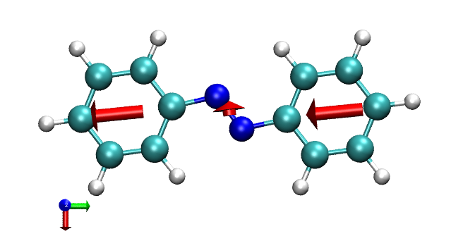
As you can see, both the two phenyl groups have significant contribution to Y component of total transition dipole moment (the red, green and blue of the axis shown at left-bottom part of the graph correspond to X, Y and Z directions, respectively). For quantitative comparison purposes, total transition dipole moment vector and its compositions are also listed below
Total:           0.1155  -2.8868  0.0
Phenyl group 1:0.14262 -1.43288 0.0
N2:             -0.16948 -0.02138 0.0
Phenyl group 2:0.14262 -1.43288 0.0
If you also want to plot total transition dipole moment as green arrow on the graph, you can input draw color green and then input dip all.
It is also possible to plot transition dipole moment contributed by each atom. To do that, we input draw delete all to remove all existing arrows, and then input dipatm, you will immediately see
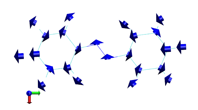
There is a very important point that should be paid attention to when using above method to decompose transition dipole moment, namely contribution of a fragment is often dependent of choice of origin, because transition charge of a fragment is often non-zero. For example, if we use subfunction 6 of hole-electron analysis module to export atomic transition charges and then sum them as fragment transition charges, you will find the value of the first phenyl group is 0.2116. Since it is non-zero, it can be proved that if overall coordinate of the azobenzene is translated, the transition dipole moment corresponding to this fragment must be varied; in other words, the result is not definite. Therefore, one should carefully discuss fragmental transition dipole moment in papers.
Another very important point is that since the transition dipole moment is decomposed via Mulliken method, the analysis method shown above will be meaningless when diffuse functions are presented in the electron excitation calculation.
4.18.13 Study electronic structure of a single excited state and difference between two excited states
Most other subsections in Section 4.18 focus on exemplifying how to study electron transition characters, however, sometimes we want to study character of a single excited state or difference between two excited states in specific property. In Multiwfn, one can perform various kinds of wavefunction analysis for an excited state as usual, however, the input file must contain wavefunction of this excited state. For multi-configuration methods that can study excited state, such as CIS and TDDFT, the excited state wavefunction must be recorded as natural orbitals (NOs), because Multiwfn always load wavefunction in terms of orbitals.
The main purpose of this section is to illustrate the function used to generate .mwfn file containing NOs of an excited state, so that we can analyze wavefunction character of this state. I strongly suggest you read Section 3.21.13 first, in which the details of generating NOs of excited states are described.
Note
There are two types of CIS/TDHF/TDA-DFT/TDDFT excited state wavefunction (or density matrix): (1) Unrelaxed density (2) Relaxed density. The difference has been detailedly described in Section 3.21.1.1. Briefly speaking, the former is not as real as the latter, but generating the latter requires additional cost (much higher than simply evaluating excitation energy). Next, I will first illustrate how to perform wavefunction analysis for an excited state and study difference between two excited states based on unrelaxed density, while at final part of this section I will also exemplify how to analyze excited state based on its relaxed density.
Example of wavefunction analysis of an excited state (based on unrelaxed density)
Here I take N-phenylpyrrole as example, assume that we want to examine Mayer bond orders for the second singlet excited state. To do so, we first carry out a regular TDDFT calculation with IOp(9/40=4) keyword, the examples\excit\N-phenylpyrrole.out is output file and examples\excit\N-phenylpyrrole.fch is corresponding .fch file. The geometry was previously optimized for ground state.
Boot up Multiwfn and input below commands
examples\excit\N-phenylpyrrole.fch
18 // Electron excitation analysis
13 // Generate natural orbitals of specific excited states
examples\excit\N-phenylpyrrole.out
2 // Choose the 2nd excited state
Now, NO_0002.mwfn has been generated in current folder, it records wavefunction of the second excited state in terms of NOs.
Reboot Multiwfn and input
NO_0002.mwfn
9 // Bond order analysis
1 // Mayer bond order
From the output you will find the bond order of the N5-C10 bond, namely the bond linking pyrrole and benzene moieties, is 0.794. If you repeat the calculation for examples\excit\N-phenylpyrrole.fch, the result will correspond to ground state, and you will find the Mayer bond order is 0.713. Clearly, the vertical excitation from S0 to S2 at minimum point of S0 weakens the strength of N5-C10 detectably.
Plotting density difference between excited states
Next I illustrate how to plot density difference between various excited states (corresponding to unrelaxed density). In fact, this is very easy, you simply need to generate Multiwfn input files containing NOs of the two excited states respectively, and then get their difference via the steps illustrated in Sections 4.5.5 or 4.18.3.
I still take N-phenylpyrrole as example. We repeat aforementioned steps using the N-phenylpyrrole.fch and N-phenylpyrrole.out to generate .mwfn files, when Multiwfn asks you to input the index of excited states, we input 1-3, then NO_0001.mwfn, NO_0002.mwfn and NO_0003.mwfn will be generated in current folder, clearly now we can study density difference between 1-2, 1-3 and 2-3.
Assume that currently we want to visualize isosurface map of electron density difference between the third and the first excited state, we reboot Multiwfn and input
NO_0003.mwfn
5 // Calculate grid data
0 // Custom operation
1 // One file will be dealt with the first loaded file
-,NO_0001.mwfn
1 // Electron density
2 // Medium-quality grid
-1 // Visualize isosurface
After setting isovalue to 0.005, we will obtain the graph below
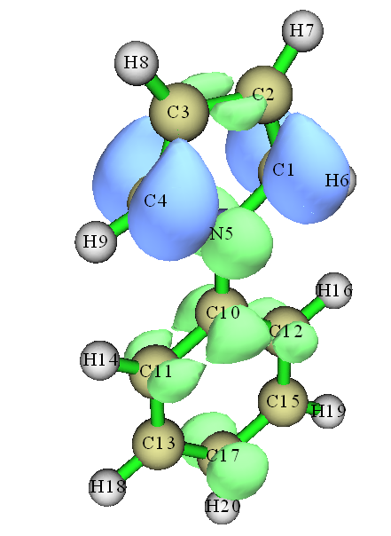
The density difference map between other excited states can be obtained similarly.
Although you can also directly use your quantum chemistry program to generate wavefunction file containing NOs for various excited states, the procedure is evidently much more cumbersome than using Multiwfn, because as shown above, the advantage of Multiwfn is that it is able to simultaneously generate .mwfn file containing NOs for a batch of excited states.
Calculate difference in fragment charge between excited states
Next, as an example, we will study difference of electron distribution at quantitative level by comparing fragment charge of the pyrrole ring between excited states 3 and 1.
Boot up Multiwfn and input
NO_0003.mwfn
7 // Population analysis
-1 // Define fragment
1-9 // The pyrrole fragment, which is composed of atoms 1~9
11 // ADCH charge
1 // Use built-in atomic densities
You will find
Namely the fragment charge of the pyrrole ring is 0.544 at the 3rd excited state. Repeat the calculation for the NO_0001.mwfn, the charge of the pyrrole ring will be found to be 0.117. The data shows that during the (hypothetical) transition from the 1st to the 3rd excited state, the pyrrole fragment will lose 0.544−0.117=0.43 electron, this well explains why in the corresponding density difference map there are obvious isosurfaces around the pyrrole ring and most of them are in blue color. Do not forget that the current result still corresponds to unrelaxed excited state density.
Wavefunction analysis of an excited state (based on relaxed density)
At final part of this section, I show how to carry out wavefunction analysis for an excited state based on its relaxed density. N-phenylpyrrole is still taken as example.
We prepare a Gaussian input file with the content below. The full file has been provided as examples\excit\N-phenylpyrrole_relaxS2.gjf.
Run this file by Gaussian, then the density matrix corresponding to relaxed density of the 2nd excited state will be written into the N-phenylpyrrole_relaxS2.chk. Then use formchk utility to convert it to N-phenylpyrrole_relaxS2.fch (which can also be directly downloaded from http://sobereva.com/multiwfn/extrafiles/N-phenylpyrrole_relaxS2.zip).
We first need to transform the density matrix to NOs. Boot up Multiwfn and input
N-phenylpyrrole_relaxS2.fch
200 // Other functions, part 2
16 // Generate NOs based on the density matrix in .fch/.fchk
CI // The label of TDDFT density matrix in the file is “CI”
y // Export new.mwfn in current folder and then automatically load it, which contains the newly generated NOs
Now the orbitals in memory have corresponded to the NOs generated based on the relaxed density of the 2nd excited state, then we can do arbitrary wavefunction analysis, for example
0 // Return to main menu
9 // Bond order analysis
1 // Mayer bond order
From the output you can find the bond order of the N5-C10 is 0.756, while as shown earlier, this value corresponding to unrelaxed density is 0.794. The small difference implies that the analysis result based on unrelaxed density is at least qualitatively correct and as useful as those derived based on the accurate but expensive relaxed density.
It is also possible to calculate density difference based on relaxed density between two excited states. You need to repeat above steps twice to respectively generate .mwfn file for two different excited states, and then get density difference as usual based on the two .mwfn files.
Note
For Gaussian users, in fact one can use such as “# PBE1PBE/6-31G* out=wfn TD(root=x)” keywords to export NOs of excited state x to specific .wfn file, which can also be employed as input file for performing wavefunction analysis of the excited state. However, do not forget that many functions in Multiwfn require basis function information, which cannot be provided by .wfn file, thus in this case the kind of analyses can used is severely limited. In addition, by solely using Gaussian it is also possible to yield and store the NOs to .fch file, as explicitly described at the beginning of Chapter 4, however this procedure is relatively cumbersome. Notice that the NOs generated in these ways correspond to relaxed excited state wavefunction. If you only need the NOs corresponding to the unrelaxed excited state wavefunction, simply adding “density=rhoci” keyword in route section.
4.18.16 Plot charge-transfer spectrum and calculate major characters of all excited states: N-phenylpyrrole as an instance
Note
Chinese version of this section is my blog article “Using Multiwfn to plot charge transfer spectrum (CTS) to intuitively analyze intrinsic characteristics of electronic spectrum” (http://sobereva.com/628), which also contains extended discussions.
If you are not familiar with IFCT analysis, please check Section 3.21.8 first to gain basic knowledge and follow Section 4.18.8 to better understand IFCT analysis via a practical example. The so-called charge-transfer spectrum (CTS), which was defined on the top of IFCT analysis, has been introduced in Section 4.21.16, please read it first before following the present example. If CTS is involved in your work, please cite Carbon, 187, 78 (2022) DOI: 10.1016/j.carbon.2021.11.005, in which I proposed CTS first time and introduced it in supplemental information.
In this section, I will exemplify how to calculate IFCT data for all excited states so that you can easily identify their major characters, then I will also illustrate how to plot CTS, which is able to intuitively reveal the nature of various peaks of UV-Vis spectrum.
The N-phenylpyrrole will be employed as an instance, five excited states were calculated by Gaussian using TDDFT at CAM-B3LYP/6-31+G(d) level. Note that IOp(9/40=4) keyword has been employed in the calculation. In this study, the phenyl group and the pyrrole group will be defined as two respective fragments, so that we can identify nature of the excited states from perspective of intrafragment electron redistribution and interfragment electron transfer.
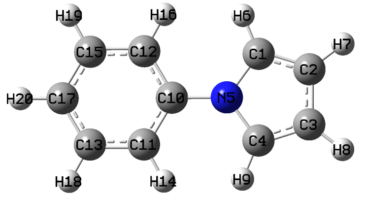
Calculate IFCT data for all excited states
Boot up Multiwfn and input
examples\excit\N-phenylpyrrole.fch // Produced by TDDFT task of Gaussian
18 // Electron excitation analysis
16 // Calculate charge-transfer spectrum and characters of all excited states
2 // Define two fragments
1-9 // Fragment 1, namely the pyrrole moiety
10-20 // Fragment 2, namely the phenyl moiety
[Press ENTER button directly] // Load examples\excit\N-phenylpyrrole.out, which is output file of Gaussian TDDFT task
2 // Hirshfeld partition (because diffuse functions were employed in the TDDFT task, Mulliken-like partition should not be used here)
Then Multiwfn starts to calculate IFCT terms for every excited state in turn, and the resulting hole and electron distributions are printed on screen. Once the calculation is finished, you will obtain IFCTdata.txt and IFCTmajor.txt in current folder, and you will also find a new subfolder "CT_multiple" (This subfolder has been provided in “examples\excit\”).
The content of IFCTdata.txt is shown below. As you can see, it contains the detailed IFCT analysis results for all excited states. The meaning of the terms is easy to understand. For example, hole(1) and ele(1) correspond to contribution of fragment 1 (pyrrole) to hole and electron distributions, respectively. redis(1) denotes amount of electron redistribution within fragment 1. 1->2 stands for amount of electron transfer from fragment 1 to fragment 2.
state  hole(1) ele(1)  hole(2) ele(2)  redis(1) redis(2)  1->2   1<-2
   1   0.5191  0.3931  0.4809  0.6069   0.2041   0.2918  0.3150 0.1890
   2   0.2452  0.0742  0.7548  0.9258   0.0182   0.6988  0.2270 0.0560
   3   0.9522  0.4356  0.0478  0.5644   0.4148   0.0270  0.5375 0.0208
   4   0.9812  0.7392  0.0188  0.2608   0.7253   0.0049  0.2560 0.0139
   5   0.9620  0.0779  0.0380  0.9221   0.0749   0.0351  0.8871 0.0030
Since there are lots of data in IFCTdata.txt, it is difficult to quickly identify major characters of excited states, especially when the number of defined fragments is more than two. Therefore, Multiwfn also exports IFCTmajor.txt, in which only the IFCT terms with contribution to each excitation larger than 5% are shown. The content of this file is
state    f     nm
   1  0.3935  245.0:  Redis(1) 20.4 %  Redis(2) 29.2 %  1->2 31.5 %  1<-2 18.9 %
   2  0.0139  244.4:  Redis(2) 69.9 %  1->2 22.7 %  1<-2  5.6 %
   3  0.0214  236.4:  Redis(1) 41.5 %  1->2 53.7 %
   4  0.0000  208.9:  Redis(1) 72.5 %  1->2 25.6 %
   5  0.1674  207.8:  Redis(1)  7.5 %  1->2 88.7 %
As you can see, oscillator strength (f), wavelength (nm) along with major IFCT terms are clearly shown. Obviously, excited state 5 (S5) mainly shows charge transfer character, while excited state 1 (S1) shows strongly mixed character. Since all other excited states have very small f, they do not notably contribute to UV-Vis spectrum.
Plot charge-transfer spectrum (CTS)
The charge-transfer spectrum (CTS) proposed by me means decomposing the total UV-Vis spectrum to individual subspectra respectively contributed by various IFCT terms, and hence the underlying nature of every noticeable peak can be graphically exhibited. To plot this kind of spectrum, we reboot Multiwfn and input
CT_multiple\CT_multiple.txt // The list file containing input files for plotting various types of CTS and corresponding legends
11 // The main function for plotting spectrum
3 // UV-Vis
0 // Plot spectrum
Now the spectrum is shown on screen. We slightly adjust plotting settings to make it look better. Close the spectrum and then input
22 // Set thickness of curves/lines/texts/axes/grid
1 // Set thickness of curves
5
0 // Return
17 // Other plotting settings
11 // Set position of legends
8 // Upper left corner
10 // Set text size of legend
45
0 // Return
3 // Set lower and upper limit of X-axis
170,300,20 // Lower limit, upper limit, and label interval
0 // Replot
The current CTS is shown below
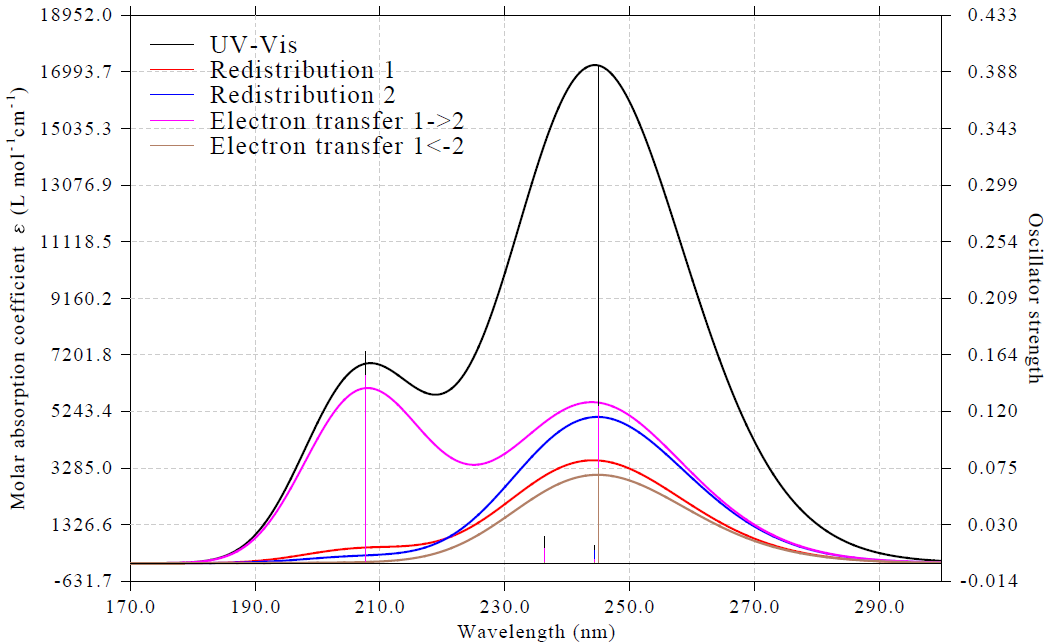
As can be clearly seen, the peak around 210 nm basically corresponds to pure charge-transfer excitation, because in this region the "Electron transfer 1->2" curve is close to the black UV-Vis spectrum curve. The highest peak at approximately 245 nm shows highly hybrid character, both the two intrafragment electron redistribution curves and the two interfragment electron transfer curves exhibit comparable heights.
The present example is relatively simple since we only defined two fragments, in fact you can define arbitrarily number of fragments. For example, if you define three fragments (e.g. respectively corresponding to D, π, A parts of a D-π-A system), then there will be 9 curves in the CTS, namely: redis(1), redis(2), redis(3), 1->2, 1->3, 2->3, 1<-2, 1<-3, 2<-3.
4.18.17 Example of performing electron density polarization analysis based on electron excitations
This section illustrates how to perform the electron density polarization analysis based on electron excitations, which was proposed in J. Phys. Chem. A, 124, 633 (2020). Please carefully read Section 3.21.17 first to gain basic knowledge. This section will reproduce the first example in the J. Phys. Chem. A paper, which employs a point charge of -0.1 e to approximately mimic the nucleophilic agent at the beginning stage of a SN2 reaction. The molecule that undergoes nucleophilic attack is CH3Cl. The distance between the point charge and the carbon is arbitrarily set to be 3 Å. See the following map for illustration.
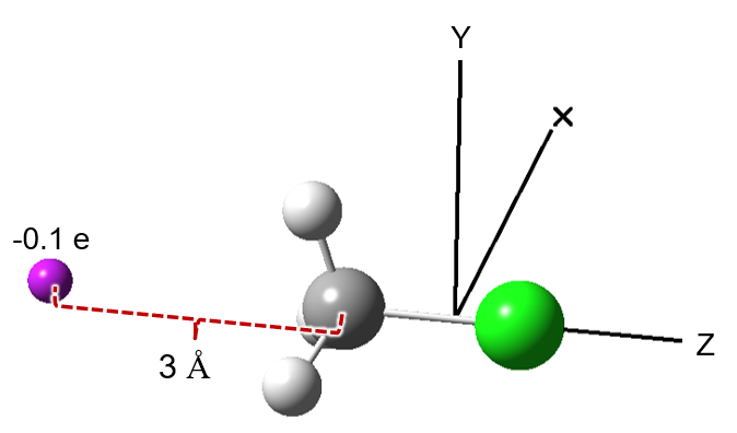
In this example we use ωB97XD/def2-TZVP level to perform TDDFT task with 50 excited states for CH3Cl by Gaussian, the geometry was optimized at B3LYP/def-TZVP level. The Gaussian input and output files have been provided in “examples\excit\CH3Cl\” folder, the .fch file converted from the resulting .chk file is provided as CH3Cl.fch. Note that IOp(9/40=4) keyword was used in the task, the necessity has been emphasized in Section 3.21.A. Since the XYZ coordinate of the carbon atom is (0.0, 0.0, -1.13395200) Å, according to the map above, evidently the point charge should be placed at (0.0, 0.0, -4.13395200) Å.
Boot up Multiwfn and input
CH3Cl.fch
18 // Electron excitation analyses
17 // Electron density polarization analysis based on electron excitations
1 // Only one point charge will be set as the external potential
0.0,0.0,-4.13395200,-0.1 // XYZ coordinate (Å) and value (e) of the point charge
2 // Medium-quality grid (corresponding to grid spacing of 0.2 Bohr. If you want to reduce cost, low-quality grid can also be used)
[Press ENTER button] // Load the Gaussian output file CH3Cl.out, which is in the same folder as the CH3Cl.fch
Now Multiwfn starts to calculate data for the 50 excited states in turn, then you will see the following output:
Excited state contributions:
  State #    Exc. Ene (Ha)       c_k          E2(kJ/mol)
       1        0.273727     -0.00000190     -0.00000000
       2        0.273727     -0.00000299     -0.00000001
       3        0.339810      0.00000105     -0.00000000
[ignored...]
      50        0.705411     -0.00008669     -0.00001392

 Excited state contributions sorted by |c_k|:
  State #    Exc. Ene (Ha)       c_k          E2(kJ/mol)
       9        0.421066      0.00755963     -0.06317769
      22        0.503194     -0.00329586     -0.01435108
      14        0.456544     -0.00278408     -0.00929093
      42        0.651216     -0.00259838     -0.01154363
      38        0.633059     -0.00208700     -0.00723935
      47        0.666453      0.00156450     -0.00428287
[ignored...]

 Total E2:   -0.001206 eV (   -0.1164 kJ/mol)
 Integral of density polarization:    5.01383559E-07
 Amount of electrons polarized:  0.01196258
It can be seen that the 9th excited state has the largest ck and contributes most to \(E^{(2)}\), so this excited state is worth examining further. “Total E2” and “Amount of electrons polarized” correspond to \(E^{(2)}\) and δN, respectively, they have small magnitude because the point charge is small and not very close to any atom.
We choose option “1 Visualize isosurface of density polarization” to visualize ρpol and then change isovalue to 0.0002, you will see the left map in the following figure, in which the green and blue colors correspond to positive (electron accumulation) and negative (electron depletion) zones, respectively. For ease of understanding, the position of the placed point charge is automatically plotted as Bq atom in the map. The ρpol obtained in this way is approximate. If you want to obtain rigorous ρpol (the right map in the following figure), you should use the common method, namely taking the difference between the electron density obtained with and without a background charge (please refer to Section 4.5.5 on how to plot electron density map), the wavefunction files generated with and without the background charge correspond to examples\excit\CH3Cl\bkchg\CH3Cl_Q.fch and the aforementioned CH3Cl.fch, respectively. It can be seen that the approximate ρpol and rigorous ρpol are in qualitative agreement with each other, indicating that the approximate ρpol estimated by means of the perturbation theory is meaningful.
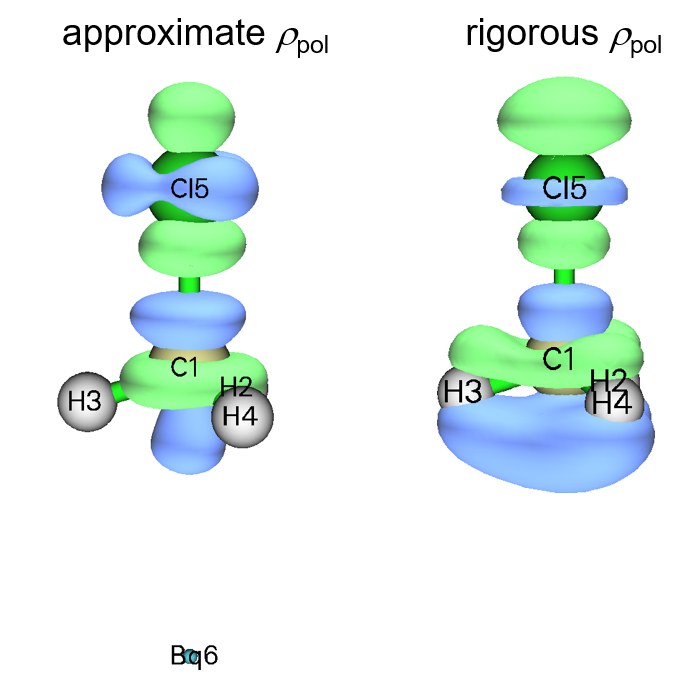
As can be seen in the figure above, there is a region with reduced electron density at the end of the Cl-C bond axis, so it can be considered that when the nucleophile carrying a local negative charge that triggers the SN2 reaction approaches the carbon atom, the carbon atom becomes more electrophilic.
Next, we choose option “2 Visualize isosurface of transition density of an excited state” and then input 9 to visualize transition density of the 9th electron excitation, which contributes most to ρpol. After setting isovalue to 0.004, you will see the following map, in which green and blue colors represent positive and negative parts, respectively. It can be seen that its distribution is fairly close to the ρpol, further confirming that the excitation from ground state to the 9th excited state has the most crucial contribution to the electron density redistribution in response to the external potential. It is worth to mention that contribution of the kth electron excitation to the ρpol is simply \(2{c}_{k}{\rho}_{0}^{k}\), where \({\rho}_{0}^{k}\) is the transition density.
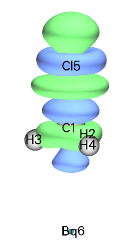
One can better understand the nature of the 9th electron excitation in terms of orbital transition picture using the NTO analysis, see Section 4.18.6 for example, or simply checking MO maps if there is a dominant MO transition. If you use the function introduced in Section 3.21.15, you will find the 9th electron excitation is dominated by (81.7%) the transition from HOMO-2 to LUMO, their isosurface maps plotted by main function 0 are shown below. It can be seen that HOMO-2 shows bonding character of C-H and C-Cl bonds, while LUMO shows antibonding character of C-Cl bond. So, we can conclude that the external perturbation by the point charge caused electron transfer from the bonding orbital to the antibonding orbital, and the C-Cl bond should hence be weakened. This speculation can be directly confirmed by calculating bond orders. The Mayer and Laplacian bond orders of the C-Cl bond calculated based on CH3Cl.fch are 1.068 and 0.432, respectively, while the values calculated for CH3Cl_Q.fch are 1.061 and 0.428, respectively, clearly indicating that the presence of the point charge detectably lowers the C-Cl bonding strength. As noted earlier, the point charge is used to mimic the nucleophilic agent at the beginning stage of the SN2 reaction of CH3Cl, our observation suggests that the electrostatic potential created by the charge borne by the nucleophile initiates the C-Cl bond breaking.
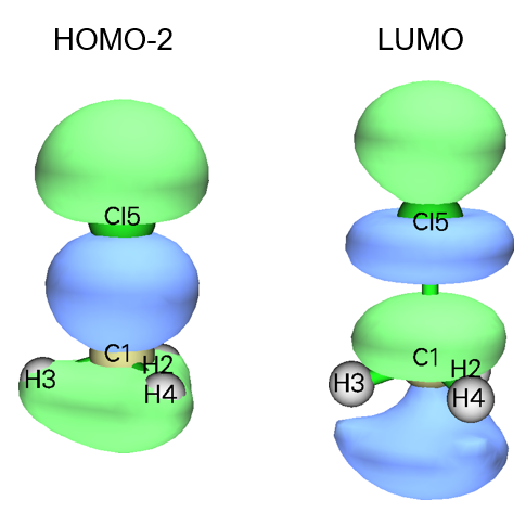
Finally, if you have interest in the distribution of the external potential, you can choose option “3 Visualize isosurface of external potential”, you will find the isosurface is spherical and exactly encloses the point charge.
From this example, we can see that the analysis of electron density polarization in terms of electron excitations indeed provides valuable and unique insight into the response of a chemical system to external perturbation. For more application instances and discussions, see J. Phys. Chem. A, 124, 633 (2020) and J. Comput. Chem., 42, 1118 (2021).
4.18.18 Example of calculating ECD/CPL dissymmetry factor (g) for (P)-[6]helicene
Please check Section 3.21.18 to understand relevant background information and the features of the function illustrated in this Section. In this section I will exemplify how to use Multiwfn to easily calculate ECD and CPL dissymmetry factor (g) for a typical chiral molecule (P)-[6]helicene, and I will also show that transition electric and magnetic dipole moments can be very conveniently visualized. TDDFT output file of Gaussian will be used for the illustration purpose, while output file of electronic excitation task of ORCA can also be used (examples\excit\g_factor\TDDFT_S0geom_ORCA.out is an example file).
Dissymmetry factor of ECD spectrum (g_CD)
examples\excit\g_factor\TDDFT_S0geom.out is output file of TDDFT task of Gaussian 16 at CAM-B3LYP/def2-SV(P) level for the helicene at its ground state structure optimized using the same level, 30 excited states were calculated, CH2Cl2 solvent environment was represented by IEFPCM solvation model. Here we will obtain \(g_{\mathrm{CD}}\) and relevant information for these states. Boot up Multiwfn, load this file, and then input
18 // Electron excitation analyses
18 // Calculate ECD/CPL dissymmetry factor (g) of chiral systems
1 // This study is for ECD
Then Multiwfn loads transition electric and magnetic dipole moments from the Gaussian output file and print them on screen, and outputs \(g_{\mathrm{CD}}\) along with various quantities closely related to it for all excited states:
 Wavlen: Wavelength (nm)
 |e_tran|: Magnitude of transition electric dipole moment (in 1E-20 esu*cm)
 |m_tran|: Magnitude of transition magnetic dipole moment (in 1E-20 erg/Gauss)
 angle: Angle between transition electric and magnetic moments (degree)
 R: Rotatory strength (in 1E-40 cgs = erg*esu*cm/Gauss)
 D: Dipole strength (in 1E-38 cgs = esu^2*cm^2)
 g: ECD dissymmetry factor (dimensionless)

 State Wavlen  |e_tran| |m_tran| angle  cos(angle)     R        D        g
    1   339.5    63.17    0.272   90.01    -0.000      0.0     39.9   0.000003
    2   320.6    28.09    0.078    0.00     1.000     -2.2      7.9  -0.011134
    3   303.5   611.95    3.922  110.89    -0.357    856.0   3745.0   0.009143
    4   288.0   106.78    0.307    0.00     1.000    -32.8    114.0  -0.011492
[ignored...]
   29   182.1   182.09    0.280  180.00    -1.000     51.0    331.6   0.006156
   30   181.8    97.30    0.811  153.75    -0.897     70.8     94.7   0.029912
It is clear that S3 should be the lowest observable excitation in both experimental ECD and UV-Vis spectra because S1 and S2 have both negligible rotatory strength (R) and dipole strength (D). It is noted that in the study work about helicene derivatives, Chem. Sci., 12, 5522 (2021), the actual S3 is even (somewhat confusingly) labelled as S1 as it is the first optically active absorption. \(g_{\mathrm{CD}}\) of S3 is 0.0091, which is in good agreement with the 0.85×10⁻² reported in Fig. 3(f) of Chem. Sci., 12, 5522 (2021).
Now we visually check transition electric dipole moment (\({\unicode{x1D6CD}}^{\mathrm{tran}}\)) and transition magnetic dipole moment (\({\mathbf{m}}^{\mathrm{tran}}\)) of S3 in VMD visualization program (http://www.ks.uiuc.edu/Research/vmd/). In the post-processing menu of the present function, choose option “2 Export current structure to .pdb file” and then input S0.pdb to generate a pdb file named “S0.pdb” in current folder, which contains the current structure. Also choose option “1 Generate VMD script file for visualizing transition electric/magnetic moments” and then input ECD.vmd to generate a script of VMD with name “ECD.vmd” in current folder.
Boot up VMD (version 1.9.3 is recommended), load the S0.pdb into it can draw the molecular structure with licorice style. Move the ECD.vmd to VMD folder and run source ECD.vmd in VMD console window to execute the script. After that, you can run emtran 3 in VMD console window to plot \({\unicode{x1D6CD}}^{\mathrm{tran}}\) and \({\mathbf{m}}^{\mathrm{tran}}\) of S3 as red and cyan arrows, respectively, as shown below. By default, the arrow lengths are 5 Å, the arrow radius is 0.15 Å. See comments at the top of ECD.vmd on how to fine-tune the plotting settings.
![Transition electric and magnetic dipole moment vectors of the S1 state of (P)-[6]helicene](../assets/figures/ch4/image1225.png)
Next, we look at S2. Both \({\unicode{x1D6CD}}^{\mathrm{tran}}\) and \({\mathbf{m}}^{\mathrm{tran}}\) of S2 state are exactly parallel to Z axis. When plotting them together in a single map, slight shifts of arrow centers must be adopted to make them visually distinguishable. In VMD console window we run this command: emtran 2 5 5 0.15 0 0.3 0 0 -0.3 0, in which “5 5 0.15” means the lengths of the two arrows are all 5 Å, and radius is 0.15 Å. “0 0.3 0” and “0 -0.3 0” mean the centers of red and blue arrows are shifted by (0.0 0.3 0.0) and (0.0 -0.3 0.0) Å, respectively. Now you can view the following map, due to the center shifts, the two arrows are not overlapping with each other.
![Transition electric and magnetic dipole moment vectors of the S2 state of (P)-[6]helicene](../assets/figures/ch4/image1226.png)
Dissymmetry factor of CPL (g_CPL)
examples\excit\g_factor\TDDFT_opt_S1.out is output file of TDDFT geometry optimization for S1 state of the helicene, S0 minimum is taken as the initial geometry. Only 3 excited states were calculated, which is adequate since the emission state of CPL is just S1 (Kasha’s rule). To obtain \(g_{\mathrm{CPL}}\), we load this file into Multiwfn, enter subfunction 18 of main function 18, Multiwfn will load the last outputted \({\unicode{x1D6CD}}^{\mathrm{tran}}\) and \({\mathbf{m}}^{\mathrm{tran}}\), which correspond to the data at S1 minimum structure. Then choose “2 This study is for CPL” You will see the following information on screen:
 State Wavlen  |e_tran| |m_tran| angle  cos(angle)     R        D        g
    1   372.4    72.32    0.226   97.32    -0.127     -2.1     52.3  -0.001592
    2   348.4    45.88    0.137  180.00    -1.000     -6.3     21.0  -0.011926
    3   334.0   748.12    3.693   73.04     0.292    805.8   5597.0   0.005759
Clearly, \(g_{\mathrm{CPL}}\) is -0.0016, which has the same sign as the experimental value -0.0009 reported in Table 1 of Commun. Chem., 1, 38 (2026) for the same molecule under the same solvent. The corresponding value reported in Fig. 3(f) of Chem. Sci., 12, 5522 (2021) is +0.0013, their calculation level is the same as ours and has very close magnitude to ours, but the sign is different. I suspect that they made mistake on the sign. The difference between the \(g_{\mathrm{CPL}}\) and \(g_{\mathrm{CD}}\) of S1 (0.000003) comes from the small structure difference between S0 and S1 minima. As illustrated earlier, you can also ask Multiwfn to export the present structure to a pdb file and export a VMD script for visualizing the \({\unicode{x1D6CD}}^{\mathrm{tran}}\) and \({\mathbf{m}}^{\mathrm{tran}}\) of S1 to provide insight into \(g_{\mathrm{CPL}}\). The files have been provided as S1.pdb and CPL.vmd in “examples\excit\g_factor\” folder.