3.2 Showing molecular structure and viewing orbitals / isosurfaces (0)¶

When main function 0 is selected, information of all atoms as well as basic information of featured orbitals (e.g. index of HOMO and LUMO, HOMO-LUMO gap) will be printed on text window, meanwhile molecular structure will be shown in a GUI window. If the input file contains orbital information, the orbitals can be viewed by selecting corresponding orbital index in the list at right-bottom corner of the window, or by directly inputting orbital index in the text box, see below screenshot. If the input file is .cub or .grd format, then one can view isosurface of the grid data in this interface.

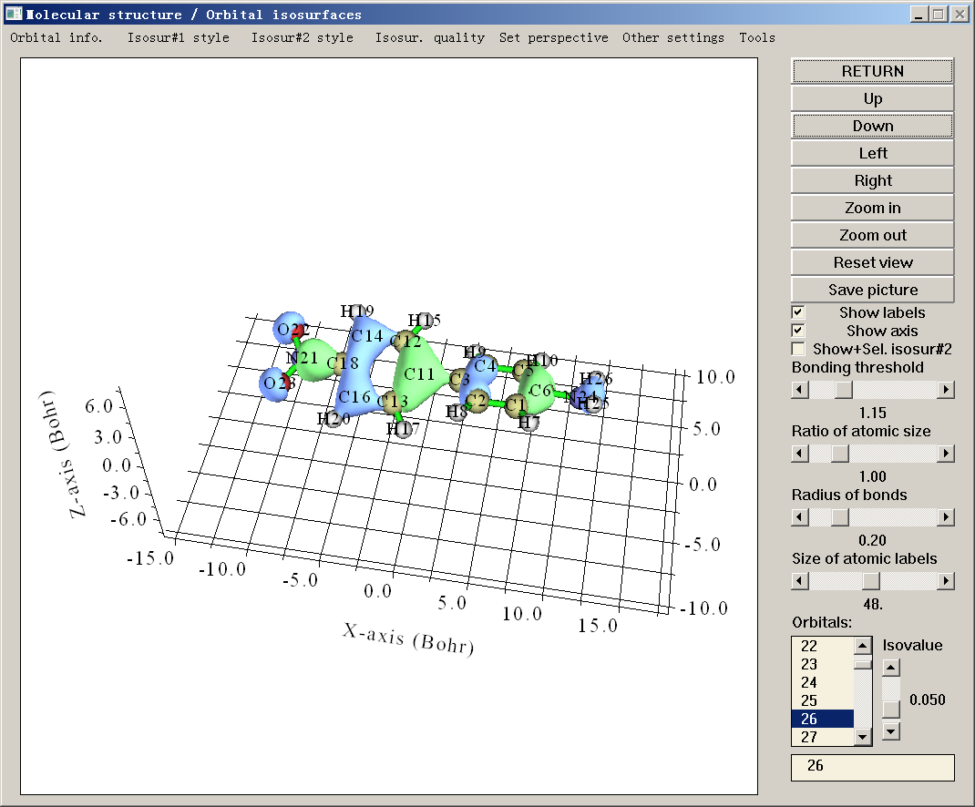
Graphical interface of main function 0

Since most widgets in this GUI are self-explanatory, I only mention some worth noting points here.

Changing viewpoint¶

Mouse dragging operations: In the drawing region, one can use the left mouse button to drag the system to freely rotate it. Holding down the Ctrl key and drag the system horizontally can rotate it along the screen. Holding down the Ctrl key and dragging the system vertically can scale the system. Holding down the Shift key and drag the system can translate it. Notice for Linux users: only after clicking the drawing region once to make the icon become a hand, the aforementioned dragging operations will be available.
Other operations: You can also rotate the viewpoint by clicking "Left", "Right", "Up", "Down" buttons at the right side of GUI. Zoom in and out can also be realized by scrolling mouse wheel in the drawing region.

To exactly set the view, one can also directly input rotation angles by selecting "Set rotation of viewpoint" option in "Set view" dropdown list in the menu, in this list there are also many other options to change view.

Changing drawing settings¶

"Ratio of atomic size" is the ratio of one-fourth of atom radius shown on screen to its van der Waals (vdW) radius, so if the slide bar is dragged to 4.0, then what to be shown is vdW surface.

There are three predefined drawing styles of system structure, you can activate one of them via “Use CPK style”, “Use vdW style” and “Use line style” in “Other settings” in the menu.

Multiwfn determines if two atoms are bonded by empirical distance criteria, if the distance between two atoms is short than 1.15 times of the sum of their CSD covalent radii, they will be considered as bonded. You can adjust this criterion by dragging "Bonding threshold" slide bar.

Note

If your input file contains connectivity information, such as .mol and .mol2, then the bonds will be displayed directly according to the provided connectivity.

The color of bonds, atomic labels and atom spheres can be set by parameters "bondRGB", "atmlabRGB" and "atmcolorfile" in settings.ini, respectively. See corresponding comments for detail. After adjusting these parameters, you need to reboot Multiwfn to make them take effect. You can also directly change atomic label color in the GUI via “Other settings”-“Set atomic label color”.

Viewing orbitals¶

By clicking "Orbital info." and then selecting corresponding options, basic orbital information can be printed on text window.

All orbital indices are listed in the right-bottom box, default selection is “none” (no orbital is shown). If you click an orbital index, Multiwfn will calculate grid data of wavefunction value for corresponding orbital, and then the orbital isosurface appears immediately. Green and blue parts correspond to positive and negative regions, respectively. The “Isovalue” slide bar controls the isovalue of the isosurface.

For efficiency consideration, the default quality of grid data is relatively coarse, the number of grid points can be set by "Isosur. quality", the larger number leads to the smoother isosurface (Note that after you adjust the number, present isosurface will be deleted). You can also set default number of grid points through changing “nprevorbgrid” in settings.ini.

For unrestricted wavefunction, the alpha and beta orbitals are recorded separately. Assume that there are \(N_{a}\) alpha orbitals and \(N_{b}\) beta orbitals, then the first \(N_{a}\) and latter \(N_{b}\) orbitals in the orbital selection list correspond to alpha and beta orbitals, respectively. Whereas in the orbital selection box, negative index corresponds to beta orbitals. For example, if you input -9, then the 9th beta orbital will be shown, and the orbital selection list will be automatically switched to the \(N_{a}\)+9 term.

Sometimes it is useful to display two orbitals simultaneously; for example, analysis of phase overlapping of two NBOs. This can be realized by "Show+Sel. Isosur#2" (Sel.=Select) check box. This check box is inactive by default, once you have chosen an orbital (corresponding isosurface will be referred to as Isosurface #1), this check box will be activated. After you clicked the check box, the isosurface of the orbital you newly selected (which will be referred to as Isosurface #2) will be shown together with the orbital you previously selected, yellow-green and purple parts correspond to positive and negative regions respectively. If the check box is deselected, Isosurface #2 will disappear, then if you reselect the check box the same Isosurface #2 will be redrawn.

The representation styles of Isosurface #1 and #2 can be adjusted by suboptions in "Isosur. #1" and "Isosur. #2" individually, available styles include solid face (default), mesh, points, solid face+mesh and transparent face. (Notice that Multiwfn cannot plot only one isosurface as transparent face). The colors for face and mesh/points can be set by corresponding suboptions too, users will be prompted to input Red, Green, Blue components for positive and negative parts in turn, the component should be between 0.0 and 1.0. For instance, 1.0,0.0,0.0 corresponds to pure red while 1.0,1.0,0.0 corresponds to Yellow. The default values for positive and negative parts can be set by "isoRGB_same" and "isoRGB_oppo" in settings.ini, respectively. Opacity for transparent face can also be customized, valid range is from 0.0 (completely transparent) to 1.0 (completely opaque).

Before showing orbital isosurfaces, Multiwfn first sets up a box internally, then calculates orbital wavefunction value at the points evenly placed in the box. The default extension distance for setting up the box is controlled by "Aug3D" parameter in settings.ini. The default value is suitable and efficient for general cases; however, in rare cases (e.g. visualizing Rydberg orbitals) you may need to manually enlarge the extension distance, you can either change the Aug3D to modify the default setting, or select "Other settings"-"Set extension distance" and then input a value to modify extension distance for present instance.

When orbital isosurface is portrayed as solid face, in rare cases the plotting effect is not quite good, for example positive and negative regions are difficult to be distinguished, in these cases you can try to adjust lighting setting by choosing "Other settings"-"Set lighting" or properly rotate the system to bypass this issue.

If you want to visualize probability density of the selected orbital instead of its wavefunction, you can choose “Other settings” - “Choose plotting wavefunction or density”, and then choose “Density”.

“Tools” submenu¶

In the "Tools" of the menu bar, there are many options:

Write settings to GUIsettings.ini: Write visualization state (e.g. color, view angle, molecular representation, text size, etc.) to GUIsettings.ini in current folder. If "Multiwfnpath" environment variable has been defined, the GUIsettings.ini will be written to the folder defined by this environment variable instead.
Load settings from GUIsettings.ini: Load visualization state from GUIsettings.ini in current folder, so that you can quickly retrieve previous visualization state. If "Multiwfnpath" environment variable has been defined, Multiwfn will first try to load this file from the folder defined by this environment variable.
Measure geometry: By inputting two, three and four atom indices in the boxes and press ENTER button, the bond length, angle, and dihedral will be returned.
Batch plotting orbitals: Via this tool you can very conveniently save a lot of selected orbitals to respective image file in current folder, see https://youtu.be/SHwrQhqBHZ0 for video illustration.
Select fragment: After selecting it and inputting an atom index, the whole fragment where the atom attributes will be highlighted, and the indices of all atoms in the fragment will be returned. This is useful when you perform some analyses, in which you need to input atom indices in the fragment of interest.
Get atom indices of a given element: Input an element name, program will return indices of all atoms corresponding to this element.
Print XYZ coordinates in Angstrom: X, Y, Z coordinates of all atoms with Å as unit will be shown in console window.
Print fractional coordinates: Fractional coordinates of all atoms will be shown in console window. This option is available only when cell information is available.
Export all internal coordinates: This option exports all bonds, angles, and dihedrals of present system to int_coord.txt in current folder. If you want to use this function with noGUI version of Multiwfn, after entering main menu, you can input geomparm, then all internal coordinates can be exported to specific file.

More functions and illustrations of the use of the main function 0 are described in Section 4.0.

Information needed

GTFs (only for viewing orbitals), atom coordinates, grid data (only for viewing isosurface of grid data)