3.200 Other functions, part 2 (200)

3.200.1 Calculate core-valence bifurcation (CVB) index and related quantities

Note

Chinese version of this section is my blog article “Using Multiwfn to calculate CVB index and measure strength of hydrogen bonds” (http://sobereva.com/461).

(1) Theory of CVB index

The idea of the so-called core-valence bifurcation (CVB) index was firstly proposed in Theor. Chem. Acc., 104, 13 (2000), this index was defined based on electron localization function (ELF) and mainly used to distinguish strength of various kinds of hydrogen bonds (H-bonds). For a H-bond of typical form (D-H⋅⋅⋅A, where D=donor, H=hydrogen, A=acceptor), this index is expressed as:

CVB index = ELF(C-V) – ELF(DH-A)

where ELF(C-V) corresponds to the ELF bifurcation value between ELF core domain and valence domain, while the ELF(DH-A) stands for the ELF value at bifurcation point between V(D,H) and V(A).

In the above-mentioned Theor. Chem. Acc. paper, the authors examined many H-bond dimers composing of HF and various kinds of monomers, it was found that the CVB index has good linear relationship with H-bond binding energy. In some succeeding papers, such as Struct. Chem., 16, 203 (2005) and J. Phys. Chem. A, 115, 10078 (2011), this point has been further confirmed, and in the former it was pointed out at CVB index “is positive in the case of weak complexes and negative in stronger ones”. In addition, in Chem. Rev., 111, 2597 (2011) the author stated that CVB index “is positive for weak hydrogen bond, and it decreases if the strength of this interaction increases; usually this index is negative for strong hydrogen bonds”.

I found the ELF(C-V) and ELF(DH-A) themselves sometimes have a better linear relationship with H-bond binding energy than CVB index, therefore I suggest you also examine this point in your practical studies when you intend to use CVB index.

(2) Manual evaluation of CVB index

Below I will show how to manually evaluate the two terms involved in the CVB index. HF⋅⋅⋅HF dimer is taken as example, the wavefunction file is provided as examples\HF_HF.wfn, it was generated at B3LYP-D3(BJ)/def2-TZVP level, the optimization was also conducted at this level. The D, H, A atoms in this system correspond to F2, H1, F3, respectively

The ELF(DH-A) term is defined unambiguously in the original paper. The topology analysis module of Multiwfn is able to locate bifurcation points of ELF, namely (3,-1) critical points of ELF. Then you can check ELF value of the bifurcation point lying between the hydrogen and acceptor atom (Section 4.2.2 illustrated how to perform topology analysis for LOL. ELF can be analyzed in similar way). However, topology analysis of ELF is time-consuming for large systems. Considering the fact that the actual ELF bifurcation point between V(D,H) and V(A) is almost exactly lying on the straight line linking H and A, it is better to use main function 3 of Multiwfn to plot an ELF curve map from the H to A and then directly read the value of corresponding minimum. Below is a screenshot of ELF topology analysis result for the HF⋅⋅⋅HF dimer

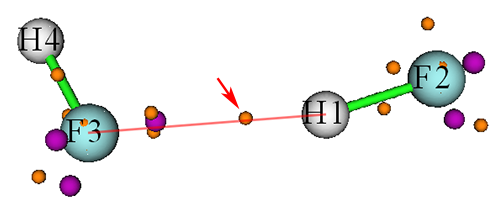
The purple and orange spheres are (3,-3) and (3,-1) type of ELF critical points (CPs), respectively. The (3,-1) CP pointed by the arrow corresponds to the aforementioned ELF bifurcation point between V(D,H) and V(A), its ELF value was found to be 0.06487, which is just the ELF(DH-A) of present system.

As can be seen from the graph above, the red linking line basically crosses the center of the orange sphere, this is why the ELF(DH-A) can also be approximately evaluated based on the ELF curve map between H1 and F3. The curve map plotted using main function 3 is shown below

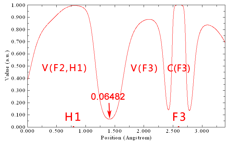
The minimum highlighted by the arrow is 0.06482, which is very close to the value 0.06487 obtained based on the expensive ELF topology analysis. This observation well demonstrates the reasonableness of employing ELF curve map between H and A to estimate the ELF(DH-A).

As regards ELF(C-V), its definition is fairly ambiguous. Since in the original paper of CVB index the authors did not explicitly and clearly explain how this quantity should be evaluated, different papers often employ different rules to calculate it, leading to serious confusion in existing literature. For example, in the CVB original paper, namely Theor. Chem. Acc., 104, 13 (2000), it seems that the ELF(C-V) was determined as maximal value at all ELF minima dissecting core and valence shell on the ELF curve between D and A atoms. However, in the subsequent paper Struct. Chem., 16, 203 (2005) written by the same author, I found the ELF(C-V) is seemingly calculated as the ELF value at one of exactly located ELF bifurcation points connecting core and valence basin of donor atom (while acceptor atom is seemingly ignored).

In my viewpoint, the best definition of ELF(C-V) should be the ELF value at the minimum dissecting core and valence shell of donor atom on the ELF curve between D and H. Again taking the HF⋅⋅⋅HF (H4-F3⋅⋅⋅H1-F2) dimer as example, the ELF curve plotted between F2 and H1 is:

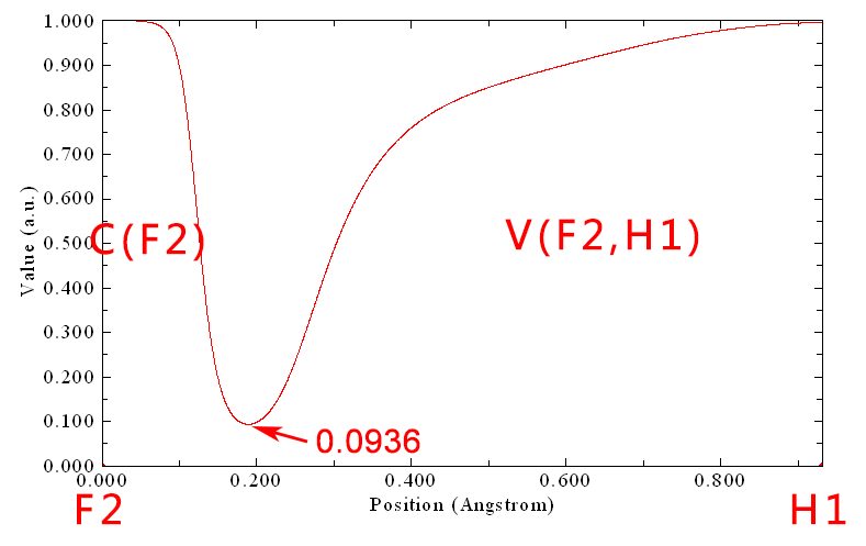
Namely ELF(C-V) = 0.0936. Hence, the CVB index for the HF⋅⋅⋅HF system should be 0.0936 − 0.0648 = 0.0288. This value is very different to the counterpart (-0.006) in Table 2 of Theor. Chem. Acc., 104, 13 (2000), because the calculation levels are different, the ways of obtaining ELF(C-V) are different, and the sign of the data in this paper was erroneously reversed.

(3) Calculating CVB index in fully automatic way

In order to simplify the calculation of CVB index in above-mentioned way as much as possible, Multiwfn provides a function used to calculate this index in fully automatic way. Still taking the HF⋅⋅⋅HF dimer as example, boot up Multiwfn and input below commands

examples\HF_HF.wfn
200  // Other function, part 2
1  // Calculate CVB index and related quantities
2,1,3  // Index of donor atom, hydrogen and acceptor atom of the H-bond, respectively

The result is

Core-valence bifurcation value at donor, ELF(C-V,D):  0.0936
Distance between corresponding minimum and the hydrogen:   0.743 Angstrom

Core-valence bifurcation value at acceptor, ELF(C-V,A):  0.1408
Distance between corresponding minimum and the hydrogen:   1.628 Angstrom

Bifurcation value at H-bond, ELF(DH-A):  0.0648
Distance between corresponding minimum and the hydrogen:   0.614 Angstrom

The CVB index, namely ELF(C-V,D) - ELF(DH-A):    0.028768

The result is completely identical to that we calculated manually. The outputted ELF(CV,A) is useless in current context, but some users may be interested in it.

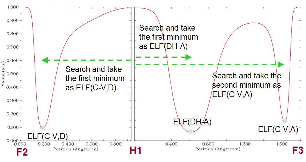
In order to make you better understand how the CVB index is automatically calculated in Multiwfn, here I explain the implementation detail. After the user inputted index of D, H and A atoms, the ELF curves corresponding to D-H and H-A are calculated in turn, and then the ELF(CV,D), ELF(DH-A) and ELF(CV-A) are automatically identified from the curve data, as illustrated below

(4) Special case: Calculating CVB index for some very strong H-bonds

In principle, the CVB index calculation protocol described above works for most kinds of systems that have typical H-bond, both intermolecular and intramolecular H-bonds can be analyzed in the same way. However, for some very strong H-bonds, whose hydrogen is lying at midpoint between two heavy atoms, such as H₂O⋅⋅⋅H⁺⋅⋅⋅OH₂, this protocol is no longer valid because its ELF curve does not show typical feature, as shown below (since the O-H-O angle in this system is close to 180°, only one plot is needed):

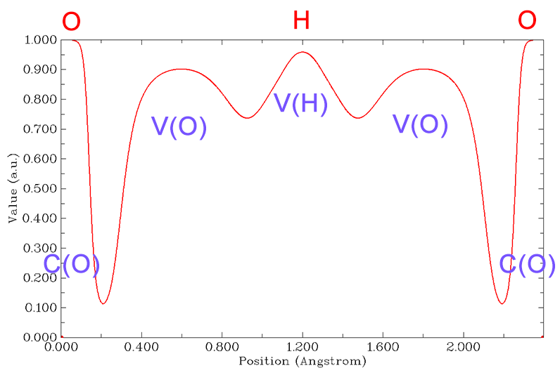
It can be seen that the V(D,H) has bifurcated as V(O) and V(H). In this case you should evaluate CVB index manually by plotting ELF curve maps, and the ELF(DH-A) in the standard CVB index expression should be replaced with the ELF value at the local minimum between the V(H) and V(O) in the curve map.

Below is a more complicated case, F^-⋅⋅⋅H⋅⋅O-H, you also need to manually evaluate the CVB index by plotting ELF curve map. The ELF curve map shown below was plotted between the F and O (the F⋅⋅⋅H⋅⋅⋅O is almost linear, therefore only one plot is needed), as can be seen the ELF is unsymmetric with respect to the central hydrogen:

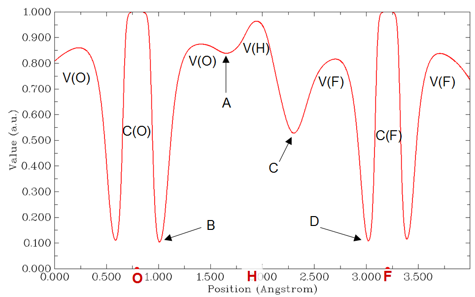
This system can be regarded as having two H-bonds, the H-bond binding energy of O-H...F and O...H-F must be very different. For the former, CVB index = ELF(B) - ELF(C), while for the latter, CVB index = ELF(D) - ELF(A). This is because when discussing the system as O-H...F (O...H-F), the O and F (F and O) behave as donor and acceptor atoms, respectively. Therefore, the minimum of point C between H and F should be regarded as the ELF(DH-A), while the minimum of point B should be viewed as ELF(C-V,D).

(5) Special case: H-bond acceptor is not a single atom

Acceptor of some H-bonds is not a single atom. For example, the acceptor of HF⋅⋅⋅ethylene is the π region of ethylene. This kind of H-bond is known as π-hydrogen bond. In this case, you also have to manually calculate the CVB index.

The wavefunction file of the HF⋅⋅⋅ethylene has been provided as examples\C2H4_HF.wfn, its geometry is shown below.

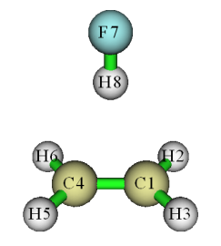
For this system, you can obtain ELF(C-V,D) by plotting ELF curve map between F7 and H8 and read the ELF value at minimum, the value will find to be 0.0944.

ELF(DH-A) of this system can be obtained via ELF topology analysis. To do this, we input below commands in Multiwfn:

2  // Topology analysis
-11  // Select the real space function to be analyzed
9  // ELF
6  // Search critical points by randomly distribute initial guesses within a sphere
4  // Set the sphere center as geometry center of three atoms
1,4,8  // Center of C1, C4 and H8 will be set as the sphere center
0  // Start searching (the sphere radius, the number of starting points can be set by corresponding options in the interface)
-9  // Return
0  // Visualize topology analysis result

Now you can see the graph below. Clearly, the critical point 5 corresponds to the bifurcation point between V(D,H) and the basin of π electron.

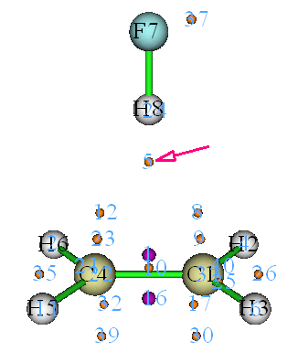
Close the GUI, select option 7, and then input 5 to check properties of the critical point 5, you will find its ELF value is 0.1241, which is just the ELF(DH-A) of this H-bond. Hence, the CVB index of this system is 0.0944 - 0.1241 = -0.0297.

Note

In fact, since this system has high symmetry, you can also obtain ELF value of the critical point 5 by simply plotting ELF curve map between H8 and midpoint of C1-C4.

Information needed

Atom coordinates, GTFs

3.200.2 Calculate atomic and bond dipole moments in Hilbert space

This function is used to calculate atomic and bond dipole moments directly based on basis functions (viz. in Hilbert space). You can also consult Section 12.3.2 of the book Ideas of Quantum Chemistry (L. Piela, 2007).

Theory

In the formalism of basis functions, the system dipole moment can be expressed as follows

\[\unicode{x1D6CD} = \unicode{x1D6CD}^{\mathrm{nuc}} + \unicode{x1D6CD}^{\mathrm{ele}} = \sum_{A} Z_{A}\mathbf{R}_{A} - \sum_{i}\sum_{j} P_{i,j}\left\langle \chi_{i} \left| \mathbf{r} \right| \chi_{j} \right\rangle\]

where Z and R are charge and coordinate of nuclei, respectively. P is density matrix, \(\left\langle \chi_{i} \left| \mathbf{r} \right| \chi_{j} \right\rangle\) is dipole moment integral between basis function i and j.

The system dipole moment can be decomposed as the sum of single-atom terms and atomic pair terms

\[\unicode{x1D6CD} = \sum_{A} \unicode{x1D6CD}_{A}^{\mathrm{tot}} + \sum_{A}\sum_{B>A} \unicode{x1D6CD}_{AB}^{\mathrm{tot}} = \sum_{A} \left( \unicode{x1D6CD}_{A}^{\mathrm{nuc}} + \unicode{x1D6CD}_{A}^{\mathrm{pop}} + \unicode{x1D6CD}_{A}^{\mathrm{dip}} \right) + \sum_{A}\sum_{B>A} \left( \unicode{x1D6CD}_{AB}^{\mathrm{pop}} + \unicode{x1D6CD}_{AB}^{\mathrm{dip}} \right)\]

The expression and physical meaning of the five terms are

\({\unicode{x1D6CD}}_{A}^{\mathrm{nuc}}\): Dipole moment due to nuclear charge

\[\unicode{x1D6CD}_{A}^{\mathrm{nuc}} = Z_{A}\mathbf{R}_{A}\]

\({\unicode{x1D6CD}}_{A}^{\mathrm{pop}}\): Dipole moment due to the electron population number localized on single atom (Notice that this is different to the electron population number calculated by Mulliken or similar methods, because the overlap population numbers have not been absorbed into respective atoms)

\[\unicode{x1D6CD}_{A}^{\mathrm{pop}} = -p_{A}^{\mathrm{loc}}\mathbf{R}_{A}\quad\quad p_{A}^{\mathrm{loc}} = \sum_{i \in A}\sum_{j \in A} P_{i,j}\left\langle \chi_{i} \left| \chi_{j} \right. \right\rangle\]

\({\unicode{x1D6CD}}_{A}^{\mathrm{dip}}\): Atomic dipole moment, which reflects the electron dipole moment around an atom. r_A is the coordinate variable with respect to nucleus A

\[\begin{gathered}\unicode{x1D6CD}_{A}^{\mathrm{dip}} = -\sum_{i \in A}\sum_{j \in A} P_{i,j}\left\langle \chi_{i} \left| \mathbf{r}_{A} \right| \chi_{j} \right\rangle\quad\quad \mathrm{where}\ \ \mathbf{r}_{A} = \mathbf{r} - \mathbf{R}_{A}\\ = -\sum_{i \in A}\sum_{j \in A} P_{i,j}\left\langle \chi_{i} \left| \mathbf{r} \right| \chi_{j} \right\rangle - \unicode{x1D6CD}_{A}^{\mathrm{pop}}\end{gathered}\]

\({\unicode{x1D6CD}}_{AB}^{\mathrm{pop}}\): Dipole moment due to the overlap population between atom A and B

\[\unicode{x1D6CD}_{AB}^{\mathrm{pop}} = -p_{AB}\mathbf{R}_{AB}\quad\quad p_{AB} = 2\sum_{i \in A}\sum_{j \in B} P_{i,j}\left\langle \chi_{i} \left| \chi_{j} \right. \right\rangle\quad\quad \mathbf{R}_{AB} = \left( \mathbf{R}_{A} + \mathbf{R}_{B} \right)/2\]

\({\unicode{x1D6CD}}_{AB}^{\mathrm{dip}}\): Bond dipole moment, which somewhat reflects the electron dipole moment around geometry center of corresponding two atoms. Of course, if A and B are not close to each other, then this term will be very small, and thus inappropriate to be called as bond dipole moment.

\[\begin{gathered}\unicode{x1D6CD}_{AB}^{\mathrm{dip}} = -2\sum_{i \in A}\sum_{j \in B} P_{i,j}\left\langle \chi_{i} \left| \mathbf{r}_{AB} \right| \chi_{j} \right\rangle\quad\quad \mathrm{where}\ \ \mathbf{r}_{AB} = \mathbf{r} - \mathbf{R}_{AB}\\ = -2\sum_{i \in A}\sum_{j \in B} P_{i,j}\left\langle \chi_{i} \left| \mathbf{r} \right| \chi_{j} \right\rangle - \unicode{x1D6CD}_{AB}^{\mathrm{pop}}\end{gathered}\]

By means of Mulliken-type partition, the bond dipole moments can be incorporated into atomic dipole moments, so that the system dipole moment can be written as the sum of single center terms

\[\unicode{x1D6CD} = \sum_{A} \left( \unicode{x1D6CD}_{A}^{\mathrm{nuc}} + \unicode{x1D6CD}_{A}^{,\mathrm{pop}} + \unicode{x1D6CD}_{A}^{,\mathrm{dip}} \right)\]

where \({\unicode{x1D6CD}'}_{A}^{\mathrm{pop}}\) is the dipole moment due to the Mulliken population number of atom A

\[\unicode{x1D6CD}_{A}^{,\mathrm{pop}} = -p_{A}^{\mathrm{Mul}}\mathbf{R}_{A}\quad\quad p_{A}^{\mathrm{Mul}} = \sum_{B}\sum_{i \in B}\sum_{j \in B} P_{i,j}\left\langle \chi_{i} \left| \chi_{j} \right. \right\rangle\]

and \({\unicode{x1D6CD}'}_{A}^{\mathrm{dip}}\) is the atomic overall dipole moment of atom A

\[\unicode{x1D6CD}_{A}^{,\mathrm{dip}} = -\sum_{B}\sum_{i \in B}\sum_{j \in B} P_{i,j}\left\langle \chi_{i} \left| \mathbf{r}_{A} \right| \chi_{j} \right\rangle = -\sum_{B}\sum_{i \in B}\sum_{j \in B} P_{i,j}\left\langle \chi_{i} \left| \mathbf{r} \right| \chi_{j} \right\rangle - \unicode{x1D6CD}_{A}^{\mathrm{Mul}}\]

Note that the B index in above formulae runs over all atoms.

Usage

The input file must contain basis function information (e.g. .mwfn, .fch, .molden and .gms).

After you enter present function, you can choose option 1 to output information of a specific atom, including: Atomic local population number, \({p}_{A}^{\mathrm{loc}}\); atomic dipole moment, \({\unicode{x1D6CD}}_{A}^{\mathrm{dip}}\); contribution to system dipole moment due to nuclear charge, \({\unicode{x1D6CD}}_{A}^{\mathrm{nuc}}\); contribution to system dipole moment due to electron, \({\unicode{x1D6CD}}_{A}^{\mathrm{dip}}+{\unicode{x1D6CD}}_{A}^{\mathrm{pop}}\); contribution to system dipole moment, \({\unicode{x1D6CD}}_{A}^{\mathrm{nuc}}+{\unicode{x1D6CD}}_{A}^{\mathrm{dip}}+{\unicode{x1D6CD}}_{A}^{\mathrm{pop}}\).

You can also choose option 2 to output information between specific atomic pair, including: bond population number, \({\unicode{x1D6CD}}_{AB}^{\mathrm{pop}}\); bond dipole moment, \({\unicode{x1D6CD}}_{AB}^{\mathrm{dip}}\); contribution to system dipole moment, \({\unicode{x1D6CD}}_{AB}^{\mathrm{pop}}+{\unicode{x1D6CD}}_{AB}^{\mathrm{dip}}\).

If choose 3, atomic overall dipole moment and related information of selected atoms will be outputted, including: Atomic Mulliken population number, \({p}_{A}^{\mathrm{Mul}}\); atomic overall dipole moment, \({\unicode{x1D6CD}'}_{A}^{\mathrm{dip}}\); contribution to system dipole moment due to nuclear charge, \({\unicode{x1D6CD}}_{A}^{\mathrm{nuc}}\); contribution to system dipole moment due to electron, \({\unicode{x1D6CD}'}_{A}^{\mathrm{dip}}+{\unicode{x1D6CD}'}_{A}^{\mathrm{pop}}\); contribution to system dipole moment, \({\unicode{x1D6CD}}_{A}^{\mathrm{nuc}}+{\unicode{x1D6CD}'}_{A}^{\mathrm{dip}}+{\unicode{x1D6CD}'}_{A}^{\mathrm{pop}}\).

If you choose option 10, then X/Y/Z components of electron dipole moment matrix will be outputted to dipmatx.txt, dipmaty.txt and dipmatz.txt in current folder, respectively. For example, the (i, j) element of Z component of electron dipole moment matrix corresponds to

\[-\sum_{i}\sum_{j} P_{i,j}\left\langle \chi_{i} \left| z \right| \chi_{j} \right\rangle\]

Information needed

Atom coordinates, basis functions

3.200.3 Generate cube file for multiple orbital wavefunctions

By this function, grid data of multiple orbital wavefunctions can be calculated and then exported to a single cube file or separate cube files at the same time.

After you entered this function, you need to first select the orbitals you are interested in (e.g. 3,5,9-17), then define grid setting, then choose the scheme to export the grid data. If you select scheme 1, then the grid data will be exported as separate files, for example orb000003.cub, orb000005.cub, orb000009.cub, etc. The number in the filename corresponds to orbital index. If you select scheme 2, then grid data of all orbitals you selected will be collectively exported to orbital.cub in current folder. Lots of visualization programs, including VMD and Multiwfn, support the cube file containing multiple sets of grid data.

For restricted and unrestricted single-determinant wavefunctions, in this function you can select orbital based on HOMO and LUMO. For example, h-3 means HOMO-3, l+2 corresponds to LUMO+2. See prompt on screen for more examples.

Information needed

Atom coordinates, GTFs

3.200.5 Plot radial distribution function for a real space function

This function is used to plot radial distribution function (RDF) for a real space function

\[RDF(r) = \int f(r,\Omega) r^{2} \mathrm{d}\Omega\]

where r is radial distance from sphere center, and Ω denotes angular coordinate in a sphere layer.

The integration curve of RDF can also be plotted

\[I(r^{\prime}) = \int_{r_{\mathrm{low}}}^{r^{\prime}} RDF(r) \mathrm{d}r = \int_{r_{\mathrm{low}}}^{r^{\prime}} \int f(r,\Omega) r^{2} \mathrm{d}\Omega\, \mathrm{d}r\]

Clearly, if \(r_{\mathrm{low}}\) is set to 0 (viz. sphere center), then I(∞) will be the integral of f over the whole space.

In present function, one can choose the real space function to be studied, set the position of sphere center, set the lower and upper limit to be calculated and plotted, set the number of points in radial and angular parts. The larger the number of points, the more accurate the integration curve.

After the parameters have been properly set, selecting option 0 to start the calculation, then you will see a new menu, in which you can plot RDF and its integration curves, save the graph or export the corresponding original data. In this menu you can also find an option used to export spherically averaged function (\(f^{\mathrm{sph}}\)), it correlates with RDF via below relationship

\[f^{\mathrm{sph}}(r) = \frac{RDF(r)}{4\pi r^{2}}\]

An example is given in Section 4.200.5.

Information needed

Atom coordinates, GTFs

3.200.6 Analyze correspondence between orbitals in two wavefunctions

Theory

This function is primarily used to analyze correspondence between the orbitals in two wavefunctions. The two sets of orbitals can be produced under different basis sets, by different theoretical methods, in different external environments, in different electronic states, or at slightly different geometries. The two sets of orbitals can also be different types, for example the first set of orbitals are canonical MOs produced by Hartree-Fock calculation, while the second set of orbitals are natural orbitals produced by post-HF calculation.

The orbitals {i} in present wavefunction (the wavefunction loaded when Multiwfn boots up) can be represented as linear combination of the orbitals {j} in another wavefunction (the wavefunction you specified after entering present module), i.e.

\(\left| i \right\rangle = \sum_{j} C_{i,j} \left| j \right\rangle\) where \(C_{i,j} = \left\langle i \middle| j \right\rangle \equiv \int \varphi_{i}(\mathbf{r}) \varphi_{j}(\mathbf{r}) \mathrm{d}\mathbf{r}\)

Once we have the overlap integral, we immediately know how j is associated with i. The contribution from orbital j to orbital i is simply the square of overlap integral, namely <i|j>²×100%. The present function is able to compute the C matrix as well as the contributions, so that you can easily make clear the relationship between the two sets of orbitals.

Usage

After you enter this function, first you need to input the orbital range to be considered for present wavefunction (istart1~iend1), then input the path of the second wavefunction and the orbital range to be considered (istart2~iend2). After that the overlap matrix between istart1~iend1 and istart2~iend2 will be calculated by Becke's multi-center numerical integration scheme. Then you will see the five largest contributions from istart2~iend2 to each orbital in istart1~iend1.

If you want to obtain all coefficients (as well as the corresponding contributions) of istart2~iend2 in a specific orbital among istart1~iend1, you can then directly input the index of the orbital.

If an orbital (i) in present wavefunction can be exactly expanded as linear combination of istart2~iend2, then the normalization condition must be satisfied:

\[\sum_{j=\mathrm{istart2}}^{\mathrm{iend2}} \left\langle i \middle| j \right\rangle^{2} \times 100\% = 100\%\]

From the Multiwfn output you can find the maximum deviation to normalization condition. If the value is zero, that means all orbitals in istart1~iend1 can be exactly represented by the orbitals in istart2~iend2.

Note that the atomic coordinate of present wavefunction and that of the second wavefunction are not necessarily identical, the two wavefunctions can even correspond to different molecules. However, if the difference of the distribution scope of the atomic coordinates in the two wavefunctions is large, the integration accuracy must be low and the result is not reliable.

Commonly the default integration grid is fine enough, i.e. 30 radial points, 302 angular points with "radcut=15". If you wish to improve the accuracy, you should set "iautointgrid" in settings.ini to 0, then you can define "radpot", "sphpot" and "radcut" in settings.ini; increasing their values will result in better integration accuracy.

The computational cost of this function directly depends on the number of orbitals in consideration; so if your system contains very large number of orbitals, do not choose all orbitals at once.

Special usage: Evaluating overlap integrals and superpositions between two sets of orbitals

Present function can also be used to evaluate overlap between orbitals, the orbitals may come from the same wavefunction, or come from two different wavefunctions.

After entering the interface of present function, if you want to obtain all overlap integrals (i.e. all <i|j>) between the above-mentioned orbitals istart1~iend1 in the first wavefunction and orbitals istart2~iend2 in the second wavefunction, simply input -1, then these integrals will be outputted to convmat.txt in current folder.

If what you need is not common overlap integral between orbital wavefunctions but overlap integral between norm of orbital wavefunctions, which is useful for measuring orbital superposition and expressed as \(\int \left| {\varphi}_{i}(\mathbf{r}) \right||{\varphi}_{j}(\mathbf{r})|\mathrm{d}\mathbf{r}\), you should input -2 in the interface of present function, then all these integrals between the orbitals istart1~iend1 and istart2~iend2 will be outputted to Snormmat.txt in current folder. Similarly, if what you need is \(\int {\left| {\varphi}_{i}(\mathbf{r}) \right|}^{2}{|{\varphi}_{j}(\mathbf{r})|}^{2}\mathrm{d}\mathbf{r}\), you should input -3 in the interface, then the result will be outputted to Snorm2mat.txt.

In fact, the present function can somewhat equivalently realize the functions introduced in Sections 3.100.5, 3.100.11 and 3.100.15, but the output format and main purpose are different.

Some usage examples of this function are given in Section 4.200.6.

Information needed

Atom coordinates, GTFs

3.200.9 Calculate average bond length and average coordinate number

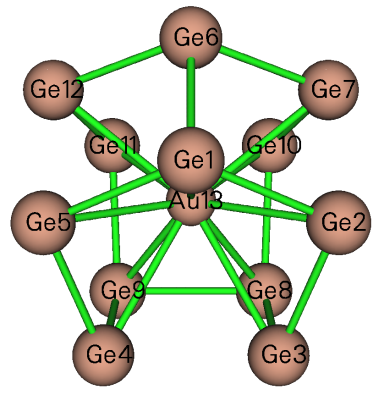
This function is used to calculate average bond length between two elements and average coordinate number. This function is particularly useful for analyzing structure character of atom clusters, for example the Ge₁₂Au cluster shown below (the structure file is provided as examples\Ge12Au.pdb). By using this function, we can immediately obtain the average Ge-Ge bond length and average Au-Ge bond length, as well as average coordinate number of Ge due to Ge-Au or Ge-Ge bonds, or of Au due to Ge-Au bonds. A nice application of this kind of analysis on Al clusters can be found in J. Chem. Phys., 111, 1890 (1999).

The average bond length is defined as follows

\[\left\langle R \right\rangle = \frac{1}{n_{\mathrm{b}}} \sum_{i>j} R_{ij}\]

where R_ij is the distance between atom i and j, only the terms smaller than or equal to a given distance cutoff (e.g. 2.2 Å) will be regarded as bonds and thus be taken into the summation. \(n_{\mathrm{b}}\) is the total number of bonds.

The average coordinate number is calculated as follows

\[CN = \frac{1}{n} \sum_{i} N_{i}\]

where N_i is the number of bonds surrounding the atom i, n is the total number of atoms.

After you entered this function, you need to input two elements, for example Ge,Au, and input a distance cutoff, for example 3.2, then the Ge-Au contacts ≤ 3.2 Å will be regarded as Ge-Au bonds and the average bond length will be calculated, the minimum and maximum bond lengths will also be outputted. After that, if you select y, the average coordinate number of Ge due to Ge-Au bonds will be shown.

Information needed

Atom coordinates

3.200.10 Output various kinds of integral between orbitals

This function is used to calculate electric/magnetic dipole moment integral, velocity integral, kinetic energy integral and overlap integral between orbitals, advanced users may recognize the significance of these data. In the case of a range of orbitals, the results are exported to orbint.txt in current folder, the first and second columns correspond to the index of the two orbitals; In the case of a pair of orbitals, the result is directly printed on screen.

The electric dipole moment integral vector between two orbitals is defined as

\[\mathbf{\unicode{x1D6CD}}_{ij} = \mathbf{\unicode{x1D6CD}}_{ji} = \left\langle \varphi_{i} \middle| -\mathbf{r} \middle| \varphi_{j} \right\rangle\]

The magnetic dipole moment integral vector between two orbitals is calculated as (more details can be found in Section 3.21.1.1. The negative sign is ignored)

\[\mathbf{M}_{ij} = i \left\langle \varphi_{i} \middle| \mathbf{r} \times \nabla \middle| \varphi_{j} \right\rangle\]

The velocity integral vector between two orbitals is evaluated as (the negative sign is ignored)

\[\mathbf{v}_{ij} = i \left\langle \varphi_{i} \middle| \nabla \middle| \varphi_{j} \right\rangle\]

It is noteworthy that, due to the Hermitian of the operators, we have

\[\begin{gathered}\mathbf{M}_{ii} = 0 \quad\quad \mathbf{M}_{ij} = {\mathbf{M}_{ji}}^{*} = -\mathbf{M}_{ji} \\\mathbf{v}_{ii} = 0 \quad\quad \mathbf{v}_{ij} = {\mathbf{v}_{ji}}^{*} = -\mathbf{v}_{ji}\end{gathered}\]

Note that the imaginary sign is not explicitly shown in the output.

The kinetic energy and overlap integrals between two orbitals are respectively evaluated as

\[K_{ij} = -\frac{1}{2} \left\langle \varphi_{i} \middle| \nabla^{2} \middle| \varphi_{j} \right\rangle \quad\quad S_{ij} = \left\langle \varphi_{i} \middle| \varphi_{j} \right\rangle\]

If you need to calculate Coulomb or exchange integral between two orbitals, you should use the function described in Section 3.200.17.

Information needed

Atom coordinates, GTFs

3.200.11 Calculate center, first/second moments, radius of gyration, and <r²> of a function

This function is used to calculate various quantities characterizing distribution of a selected real space function.

Theory

The center of a real space function f is defined as

\[\mathbf{r}_{c} = \frac{\int \mathbf{r} \times f(\mathbf{r}) \mathrm{d}\mathbf{r}}{\int f(\mathbf{r}) \mathrm{d}\mathbf{r}}\]

where the integral is performed over the whole space.

The first moment is a vector and is evaluated as

\[\mathbf{\unicode{x1D6CD}} = \begin{bmatrix} \mu_{x} \\ \mu_{y} \\ \mu_{z} \end{bmatrix} = \int \begin{bmatrix} x \\ y \\ z \end{bmatrix} f(\mathbf{r}) \mathrm{d}\mathbf{r}\]

where x, y, z are the Cartesian coordinate components relative to r_c.

The second moment is a matrix and defined as

\[\mathbf{\Theta} = \begin{bmatrix} \Theta_{xx} & \Theta_{xy} & \Theta_{xz} \\ \Theta_{yx} & \Theta_{yy} & \Theta_{yz} \\ \Theta_{zx} & \Theta_{zy} & \Theta_{zz} \end{bmatrix} = \int \begin{bmatrix} x^{2} & xy & xz \\ yx & y^{2} & yz \\ zx & zy & z^{2} \end{bmatrix} f(\mathbf{r}) \mathrm{d}\mathbf{r}\]

If its eigenvalues {ε} are sorted from low to high, then the anisotropy of Θ can be calculated as \(\varepsilon_{3} - \left( \varepsilon_{1} + \varepsilon_{2} \right) / 2\). The radius of gyration is calculated as \(\sqrt{\frac{\varepsilon_{1} + \varepsilon_{2} + \varepsilon_{3}}{\int f(\mathbf{r}) \mathrm{d}\mathbf{r}}}\).

Spatial extent \(\left\langle {r}^{2} \right\rangle=\int ({x}^{2}+{y}^{2}+{z}^{2})f(\mathbf{r})\mathrm{d}\mathbf{r}\) is simply the trace of the second moment matrix, or the sum of its three eigenvalues. If f(r) is chosen to be electron density, then <\(r^2\)> corresponds to the well-known electronic spatial extent (ESE). Note that ESE and electric dipole/multipole moments can be evaluated analytically and much more efficiently by a specific function in Multiwfn, see Section 3.300.5.

Usage

This function employs Becke's multicenter integration method for evaluating above-mentioned quantities. The accuracy is fully determined by radial points and angular points, which can be set by "radpot" and "sphpot" in settings.ini, respectively.

Option 1 calculates and outputs all aforementioned quantities. The real space function to be studied can be selected by option 3. The center (r_c) defaults to (0,0,0), and it can be manually set by option 4. Option 2 is used to evaluate the center of the selected real space function, which can be directly taken as the r_c for the subsequent calculation of option 1 (evidently, if r_c is set to be the center of the selected function, the calculated first moment will be zero).

When using option 1, if the real space function to be studied is chosen as electron density, then the nuclear contribution of quadrupole moment and molecular quadrupole moment tensors will also be outputted. In fact, the latter can be straightforwardly obtained by subtracting the former by the second moment of electron density.

If the real space function of interest has both positive and negative parts with comparable magnitude (e.g. orbital wavefunction with evident positive and negative phases), option 5 is usually recommended to use instead of option 2 for evaluating the distribution center of the selected real space function, because option 5 uses absolute function value in the evaluation, therefore cancellation effect can be avoided. In addition, for such kind of real space function, in order to calculate their aforementioned statistical quantities, it is suggested to choose option -1 once before choosing option 1, in this case the absolute function value will be used in the evaluation.

A brief example is given here. To evaluate the first and second moments of spin density (relative to the center of spin density), after loading a wavefunction file, you should input

200  // Other function (Part 2)
11  // The present function
3  // Select a real space function
5  // Spin density
2  // Calculate center of spin density
y  // Take the calculated center for evaluating various data in option 1
1  // Evaluate various data for spin density

Then the data will be shown on screen.

See my blog article “Using Multiwfn to exhibit excess electrons and calculate their radius of gyration” (http://sobereva.com/658, in Chinese) for more illustration of using this module.

Information needed

Atom coordinates, GTFs

3.200.12 Calculate energy index (EI) or bond polarity index (BPI)

This function is used to calculate energy index (EI) and bond polarity index (BPI), which were defined in J. Phys. Chem., 94, 5602 (1990) and further discussed in J. Phys. Chem., 96, 157 (1992).

The EI for atom A in a molecule is defined as follows

\[\mathrm{EI}_{A} = \frac{\sum_{i}^{\mathrm{val}} \varepsilon_{i} \eta_{i} \Theta_{i,A}}{\sum_{i}^{\mathrm{val}} \eta_{i} \Theta_{i,A}}\]

where Θ_i,A denotes composition of atom A in MO i. η_i and ε_i are occupation and energy of MO i, respectively. The summation runs over valence MOs. In fact, the denominator is simply the number of valence electrons of atom A, and the numerator corresponds to total energy of its valence electrons. Therefore, EI_A can be regarded as average energy per valence electron of atom A. In the original paper of EI, Mulliken method was used to compute the atomic contribution to MOs, thus this method is also employed in present implementation of EI, though other methods such as Hirshfeld partition should work equally well or even better. (Note that since Mulliken method is used, which is incompatible with diffuse functions, the use of diffuse basis functions must be avoided!)

The BPI between atoms A and B in a molecule is defined as

\[\mathrm{BPI}_{AB} = \left( \mathrm{EI}_{A} - \mathrm{EI}_{A}^{\mathrm{ref}} \right) - \left( \mathrm{EI}_{B} - \mathrm{EI}_{B}^{\mathrm{ref}} \right)\]

where EI^ref is reference EI value derived from calculation of homonuclear species. For example, you study BPI_CN for H₃C-NH₂, then \({\mathrm{EI}}_{\mathrm{C}}^{\mathrm{ref}}\) is computed as EI_C in ethane, and \({\mathrm{EI}}_{\mathrm{N}}^{\mathrm{ref}}\) is computed as EI_N in H₂N-NH₂. The larger magnitude of BPI_AB implies higher bond polarity of the A-B bond.

Group electronegativity is evaluated as negative of EI_X for corresponding radical, X is the attaching atom. For example, to obtain group electronegativity for -CH₃ group, you should calculate -EI_C for ⋅CH₃ radical.

This function of Multiwfn is used to calculate EI for specific atoms in present system, all the R, RO and U types of HF/DFT wavefunction are supported. Multiwfn automatically detects the number of inner-core electrons and determines which MOs are the valence ones and thus should be taken into account.

An example is given in Section 4.200.12.

Information needed

Atom coordinates, basis functions

3.200.13 Evaluate orbital contributions to density difference or other grid data

Theory

This function is mainly designed to evaluate contribution of each of selected orbitals to a given density difference, Δρ, so that you can clearly understand which orbital(s) are main contributor(s) of change in electron density distribution. A similar idea has been employed in J. Mol. Model., 24, 25 (2017) to study contribution of various NBO orbitals to Fukui function (a special kind of electron density, see Section 4.5.4) to better unravel its chemical meaning. Below, the theory and algorithm used in the present function are outlined.

Δρ is able to be approximately represented as linear combination of probability density of orbitals, which is norm of corresponding orbital wavefunction

\[\Delta\rho(\mathbf{r}) \approx \sum_{i} p_{i} \left| \varphi_{i}(\mathbf{r}) \right|^{2}\]

What we need to obtain is the optimal value of {p} for expanding the Δρ. The p_i can be regarded as contribution of orbital i to the Δρ. The {p} could be derived via least-squares method by minimizing the difference between Δρ and \(\sum_{i} p_{i} \left| \varphi_{i}(\mathbf{r}) \right|^{2}\) over the whole space, at the meantime the sum of {p} could be constrained to a given value P via Lagrangian multiplier technique. The error function to be minimized in the actual implementation is

\[F = \int \left[ \Delta\rho(\mathbf{r}) - \sum_{i} p_{i} \left| \varphi_{i}(\mathbf{r}) \right|^{2} \right]^{2} \mathrm{d}\mathbf{r} + \lambda \left[ \sum_{i} p_{i} - P \right]\]

In Multiwfn, the integral is treated as numerical integration based on evenly distributed grids, that is

\[F = \Delta_{V} \sum_{\mu} \left[ \Delta\rho(\mathbf{r}) - \sum_{i} p_{i} \left| \varphi_{i}(\mathbf{r}) \right|^{2} \right]^{2} + \lambda \left[ \sum_{i} p_{i} - P \right]\]

where µ is index of grid point, Δ_V is grid volume.

Clearly, the conditions below should be satisfied to determine the optimal {p}

\[\begin{gathered} \frac{\partial F}{\partial p_{i}} = 0 \quad\quad i = \{1,2,3...\} \\ \sum_{i} p_{i} = P \end{gathered}\]

more explicitly,

\[\frac{\partial F}{\partial p_{i}} = 0 \Rightarrow \sum_{j} p_{j} \sum_{\mu} \left| \varphi_{i}(\mathbf{r}_{\mu}) \right|^{2} \left| \varphi_{j}(\mathbf{r}_{\mu}) \right|^{2} + \lambda = \sum_{\mu} \left| \varphi_{i}(\mathbf{r}_{\mu}) \right|^{2} \Delta\rho(\mathbf{r}_{\mu})\]

Obviously, the working equation to determine {p} should be

\[\begin{gathered} \begin{bmatrix} A_{1,1} & \cdots & A_{1,N} & 1 \\ \vdots & \ddots & \vdots & \vdots \\ A_{N,1} & \cdots & A_{N,N} & 1 \\ 1 & 1 & 1 & 0 \end{bmatrix} \begin{bmatrix} p_{1} \\ \vdots \\ p_{N} \\ \lambda \end{bmatrix} = \begin{bmatrix} B_{1} \\ \vdots \\ B_{N} \\ P \end{bmatrix} \\ A_{i,j} = A_{j,i} = \sum_{\mu} \left| \varphi_{i}(\mathbf{r}_{\mu}) \right|^{2} \left| \varphi_{j}(\mathbf{r}_{\mu}) \right|^{2} \\ B_{i} = \sum_{\mu} \left| \varphi_{i}(\mathbf{r}_{\mu}) \right|^{2} \Delta\rho(\mathbf{r}_{\mu}) \end{gathered}\]

The fitting error reported by Multiwfn is estimated using the following formula

\[\begin{gathered} \mathrm{definition\ 1}: \int \left| \Delta\rho(\mathbf{r}) - \sum_{i} p_{i} \left| \varphi_{i}(\mathbf{r}) \right|^{2} \right| \mathrm{d}\mathbf{r} \\ \mathrm{definition\ 2}: \int \left( \Delta\rho(\mathbf{r}) - \sum_{i} p_{i} \left| \varphi_{i}(\mathbf{r}) \right|^{2} \right)^{2} \mathrm{d}\mathbf{r} \end{gathered}\]

In principle, this algorithm works for any kind of Δρ and orbital. For example, the Δρ may correspond to Fukui function, density variation during electron excitation and so on. The orbital could be localized molecular orbital (LMO), NBO, MO, etc. The contribution p can be positive or negative, the sign reflects phase of participation of orbital density in the Δρ. Notice that the choice of orbital range is highly arbitrary while evidently affects the result. For example, the range can include all orbitals of a certain type, or only include occupied ones.

Usage

Below is the common procedure to derive contribution of a set of orbitals to Δρ via the present function

• (1) Use Multiwfn or other codes to generate cube file of Δρ. The procedure of calculating grid data of Δρ has been substantially illustrated in many sections of present manual, for example, Section 4.5.4 (Fukui function and dual descriptor) and Section 4.18.3 (Δρ corresponding to electron excitation).

• (2) Load a file containing orbitals of interest into Multiwfn, then enter subfunction 13 of main function 200.

• (3) Input the path a cube file containing Δρ to make Multiwfn load it.

• (4) Use option 1 to set the constraint on the sum of contributions, namely the P value in above equations. The P is default to 1.0.

• (5) Select option 0, then set the range of orbitals to be taken into account. After calculation, contribution (p) of all chosen orbitals will be shown on screen.

• (6) In the post-processing menu, you can choose to visualize isosurface of Δρ, fitted density \(\sum_{i} p_{i} \left| \varphi_{i}(\mathbf{r}) \right|^{2}\) or their difference \(\Delta\rho - \sum_{i} p_{i} \left| \varphi_{i}(\mathbf{r}) \right|^{2}\) so that you can visually examine the fitting quality. The fitted density can also be exported as cube file.

In Multiwfn, there are two modes to deal with the grid data of orbitals during construction of the A matrix and B vector. You can switch the mode via option 2.

• Memory based (default): Grid data of density of all chosen orbitals are automatically calculated first and recorded in memory, in this case the calculation is fairly fast however the requirement on available memory is very high when large range of orbitals is selected and the grid quality is relatively high. This mode is strongly recommended to use if Multiwfn does not crash due to insufficient memory.

• Cube file based: Grid data of density of all chosen orbitals are automatically calculated and saved as individual cube files in current folder as rho_xxxxx.cub, where xxxxx is orbital index. The file will be loaded when corresponding orbital is used to construct the A matrix and B vector. The speed of this mode is by far slower than the "memory based" mode, but the advantage is that memory consumption is almost negligible.

  Note that the grid setting of the automatically calculated orbital densities is set by the program to exactly identical to that of the loaded Δρ grid data.

It is important to note that the present function is general, flexible and not necessarily limited to study orbital contributions to Δρ. For example, if the provided cube file contains grid data of ρ rather than Δρ, then the present function will yield contribution of selected orbitals to ρ (of course, before doing this, the P should be properly set to make the resulting contribution values meaningful. If you are not sure how to set it, you can simply remove the constraint)

Practical analysis examples of this function are given in Section 4.200.13.

3.200.14 Domain analysis (obtaining properties within isosurfaces of a function)

This function is used to integrate specific real space functions in domains. The domains refer to individual spatial regions enclosed by isosurfaces of a specific real space function. For example, you can use this function to integrate electron density within various domains defined by isosurfaces of reduced density gradient (RDG) to study strength of weak interactions at different places. If this module is flexibly utilized, many special analyses can be realized. For example, visualizing and obtaining volume of molecular cavity (see Section 4.200.14.2 for example).

Basic usage

Below is basic procedure of using this module:

(1) After entering the domain analysis module, use options 2 and 3 to set the way to define the domains. For example, you selected RDG by option 2 and inputted <0.5 in option 3, then the regions where RDG is smaller than 0.5 will be identified as different domains.

Note that periodicity can be taken into account during identification of domains. To enable it, choose option “4 Toggle considering periodicity during domain analysis” to set its status to “Yes”.

(2) Choose option 1 and properly define grid, then Multiwfn starts to calculate the grid data for the real space function you selected and identifies domains that satisfied the criterion you set.

NOTE: If you already have grid data in memory, for example you just calculated it via main function 5 or directly load a .cub file when Multiwfn boots up, you can also choose option -1 to directly use the grid data instead of calculating a new grid data. In this case, option 2 is evidently meaningless.

(3) Once calculation in last step is finished, Multiwfn prints total number of grids in each domain. In very simple case, from this information you may directly infer which domains are those you want to study, while for general cases, you need to use option "3 Visualize domains" to visualize domains in a GUI window, in which you can select domain at the right-bottom list and check its profile, each green point on the graph corresponds to a grid in the domain.

Once you have found the domains of interest, and you want to integrate a real space function in a domain, you can choose option "1 Perform integration for a domain", then you will be asked to input index of the domain, and then select the integrand. The integrand can be (1) An arbitrary real space function supported by Multiwfn (2) The grid data currently stored in memory (3) The grid data recorded in a .cub file (you will be asked to input its path. The grid distribution in this file must be exactly identical to that of present grid data). After performing the integration, the integral value, domain volume and average/maximum/minimum value of the integrand in the domain will be outputted. In addition, minimum and maximum X/Y/Z of grids belonging to the domain, as well as span distance in X/Y/Z will also be outputted. You can also select option "2 Perform integration for all domains" to obtain integral values for all domains at once. (Hint: If what you need is just domain volume, you can choose the user-defined function as integrand, which by default is 1.0 everywhere and thus integrating this function does not take any computational time).

In addition, some regions that you are interested in may be identified as separated domains, to study the property of the regions more conveniently, you can choose option "-1 Merge specific domains" to merge selected domains as a single domain, so that you do not need to manually sum up their integral values.

Via option 12 in post-process menu, you can export X, Y, Z coordinates along with value of grid data of all grids in specific domain to domain.txt in current folder.

Visualizing domains by third-part tool

If you wish to visualize domains in third-part programs such as VMD, there are two ways:

• Select "10 Export a domain as domain.cub file in current folder" and input index of the domain of interest, then Multiwfn will export the domain as domain.cub, in which the grid point belonging and not belonging to the domain have value of 1 and 0, respectively (value of boundary grids are also outputted as 0 to guarantee that the isosurfaces always look closed). After that, you can load the cube file into visualization program to visualize isosurface using isovalue of 0.5.

• Select "11 Export boundary grids of a domain to domain.pdb file in current folder" and input index of the domain of interest, then the resulting .pdb file will contain particles, each one corresponds to a boundary grid. You can directly drag this file into VMD and render the particles as spheres to visualize domain.

Special usage: Studying interactions

In the post-processing menu, there is an option "5 Calculate q_bind index for a domain", this is used to calculate the \(q_{\mathrm{bind}}\) index defined in J. Phys. Chem. A, 115, 12983 (2011), in which it was demonstrated that for hydrogen-bond dimer, the scan curve of \(q_{\mathrm{bind}}\) index well mimics to actual potential energy curve. This index for a domain is defined as:

\[\begin{gathered} q_{\mathrm{att}} = \int_{\lambda_{2}(\mathbf{r}) < 0} \rho^{n}(\mathbf{r}) \mathrm{d}\mathbf{r} \quad\quad \mathrm{attractive\ effect} \\ q_{\mathrm{rep}} = \int_{\lambda_{2}(\mathbf{r}) > 0} \rho^{n}(\mathbf{r}) \mathrm{d}\mathbf{r} \quad\quad \mathrm{repulsive\ effect} \\ q_{\mathrm{bind}} = -\left( q_{\mathrm{att}} - q_{\mathrm{rep}} \right) \end{gathered}\]

where λ₂(r) is the second largest eigenvalue of electron density Hessian matrix at r, its sign can be utilized to discriminate interaction type. The paper showed that n = 4/3 gives best correlation between \(q_{\mathrm{bind}}\) and actual potential curve. In Multiwfn the n can be manually set. Note that the paper used isosurface of RDG = 0.6 when calculating this index. More negative of \(q_{\mathrm{bind}}\) may imply more stable interaction.

It is noteworthy that in the post-processing menu there is a very flexible option "Perform integration for subregion of some domains according to range of sign(lambda)*rho", which may be useful in studying interactions. You can first select a batch of domains, and then define which subregions of the domains will be integrated by setting range of sign(λ₂)ρ (if you are not familiar with it, check Section 3.23.1), the real space function as integrand can be arbitrarily chosen. After calculation, integral of the selected real space function and volume of the subregion of each considered domain will be outputted in turn; in addition, the result for the areas with positive and negative λ₂ in the subregions is also individually printed. Via this option, you can realize special aim, for example, obtaining integral of kinetic energy density within the subregion where sign(λ₂)ρ is between -0.015 and 0.015 a.u. for the RDG < 0.6 domain corresponding to an intermolecular interaction region.

About integration accuracy

The method used to integrate domains in present module is even-grid integration method. In other words, the integration value of a real space function for a domain is simply the sum of the real space function value of the grids constituting the domain multiplied by grid volume. Therefore, the accuracy of integration result is directly affected by the quality of grid you set.

Illustrative application examples of present module are given in Section 4.200.14.

3.200.15 Calculate electron correlation index

The total, dynamic and nondynamic electron correlation indices proposed by Matito et al. in Phys. Chem. Chem. Phys., 18, 24015 (2016) are useful indicators of measuring magnitude of electron correlation in present system.

Dynamic and nondynamic electron correlation indices (\(I_{\mathrm{D}}\) and \(I_{\mathrm{ND}}\)) are defined as

\[\begin{gathered} I_{\mathrm{D}} = \frac{1}{4} \sum_{i} \left\{ \left[ \eta_{i}(1-\eta_{i}) \right]^{1/2} - 2\eta_{i}(1-\eta_{i}) \right\} \\ I_{\mathrm{ND}} = \frac{1}{2} \sum_{i} \eta_{i}(1-\eta_{i}) \end{gathered}\]

where i denotes index of natural spin orbital, η is corresponding occupation number. Note that in some cases, η may be marginally larger than 1.0 or negative, Multiwfn automatically set it to 1.0 and 0.0 respectively to make the calculation feasible.

Total electron correlation index defined is

\[I_{\mathrm{T}} = I_{\mathrm{D}} + I_{\mathrm{ND}} = \frac{1}{4} \sum_{i} \sqrt{\eta_{i}(1-\eta_{i})}\]

Present function is used to calculate all the three electron correlation indices. Any wavefunction file carrying occupation number of natural orbitals may be used as input file, e.g. .mwfn, .wfn, .wfx and .molden files. An example is given in Section 4.A.6.

Note that Matito et al. also proposed local version of the three functions to characterize electron correlation in local regions, Multiwfn is also able to study them, see Section 4.A.6 for example.

3.200.16 Generate natural orbitals, natural spin orbitals (NSO) and spin natural orbitals (SNO) based on the density matrix in .fch/.fchk file

In .fch (or .fchk) file, density matrix is always recorded. For example, if you carried out an MP2 task for an open-shell system with Gaussian keywords "# MP2/cc-pVTZ density", then the resulting .fch file will have below four fields recording corresponding type of density matrix:

Total SCF Density, Spin SCF Density, Total MP2 Density, Spin MP2 Density

While for a closed-shell system, if the keyword used is "# TD PBE1PBE/6-311G* density", then the resulting .fch file will contain below type of density matrix:

Total SCF Density, Total SCF Density, Total CI Rho(1) Density, Total CI Density

If you do not know which kinds of density matrix are recorded in the .fch file, simply search "Density" in the file.

Various kinds of natural orbitals can be obtained via diagonalization of proper type of density matrix:

• Natural orbitals (NOs): Diagonalizing total density matrix. The occupation is from 0.0 to 2.0. This type of NOs is also known as spatial NOs, and specifically, unrestricted natural orbital (UNO) for unrestricted wavefunctions

• Alpha and beta natural orbitals (collectively known as natural spin orbitals, NSOs): Diagonalizing alpha and beta density matrix, respectively. The occupation is from 0.0 to 1.0.

• Spin natural orbitals (SNOs): Diagonalizing spin density matrix (i.e. Difference between alpha and beta density matrix). The occupation is from -1.0 to 1.0. The SNO with positive (negative) occupation represents distribution of unpaired alpha (beta) electrons.

Using the present function, you can obtain any set of above-mentioned types of NOs. For example, if you want to obtain SNOs of triplet water at CCSD/cc-pVDZ level, you can run below Gaussian input file:

%chk=C:\CCSD_water_m3.chk
#p CCSD/cc-pVDZ density

test

0 3
O 0.00000000     0.00000000     0.11930801
H 0.00000000     0.75895306    -0.47723204
H 0.00000000    -0.75895306    -0.47723204

Convert the .chk file to .fch, then boot up Multiwfn and input

C:\CCSD_water_m3.fch
200
16
CC   // Meaning that we want to analyze coupled-cluster density matrix. You can also input SCF here to analyze Hartree-Fock density matrix
3  // Generate SNOs (if the system is closed-shell, this selection will not occur, since only NOs can be generated in this case)

Now the basis function information in memory has been updated to SNOs. If then you want to visualize SNOs, or to perform real space function analysis (e.g. analyzing orbital composition of SNOs via Hirshfeld partition), you should choose y to export wavefunction information to new.mwfn in current folder, and then program will automatically load it. After that, all subsequent analyses will correspond to SNOs.

One of my blog articles detailedly discussed and presented analysis example of SNOs: "The way of generating natural orbitals based on fch file in Multiwfn and analysis instances about excited state wavefunctions and spin natural orbitals" (in Chinese) http://sobereva.com/403.

Note: Once .mwfn file containing SNOs is loaded into Multiwfn, the system will be regarded as open-shell and there will be the same number of alpha and beta orbitals, only the former corresponds to SNOs, while the latter are completely meaningless and you should simply ignore them.

This function works well for .fch/.fchk files produced by Gaussian and PSI4, and may or may not be compatible with other programs.

If this function is used in combination with PSI4, you can analyze wavefunction as high as CCSD(T) level, please check Section 4.A.8 for detail.

The example in Section 4.18.9 utilized this function to generate natural orbitals for transition density matrix.

Information needed

.fch/.fchk file

3.200.17 Calculate Coulomb and exchange integral between two orbitals

Theory and implementation

Coulomb (ii|jj) and exchange integral (ij|ji) are the two most important integrals in quantum chemistry. This function is used to calculate them between two selected orbitals i and j, their expressions are:

\[\begin{gathered} \left( ii \middle| jj \right) = \int\!\!\int \frac{\varphi_{i}^{*}(\mathbf{r}_{1})\varphi_{i}(\mathbf{r}_{1})\varphi_{j}^{*}(\mathbf{r}_{2})\varphi_{j}(\mathbf{r}_{2})}{r_{12}} \mathrm{d}\mathbf{r}_{1} \mathrm{d}\mathbf{r}_{2} \\ \left( ij \middle| ji \right) = \int\!\!\int \frac{\varphi_{i}^{*}(\mathbf{r}_{1})\varphi_{j}(\mathbf{r}_{1})\varphi_{j}^{*}(\mathbf{r}_{2})\varphi_{i}(\mathbf{r}_{2})}{r_{12}} \mathrm{d}\mathbf{r}_{1} \mathrm{d}\mathbf{r}_{2} \end{gathered}\]

This function is applicable for any kind of orbital, such as molecular orbitals, localized molecular orbitals, natural transition orbitals and so on.

Currently, the integral is calculated based on uniform grid (i.e. evenly placed grid):

\[\begin{gathered} \left( ii \middle| jj \right) = (d_{\mathrm{x}} d_{\mathrm{y}} d_{\mathrm{z}})^{2} \sum_{k} \varphi_{i}^{2}(\mathbf{r}_{k}) \sum_{l \neq k} \frac{\varphi_{j}^{2}(\mathbf{r}_{l})}{\left| \mathbf{r}_{l} - \mathbf{r}_{k} \right|} \\ \left( ij \middle| ji \right) = (d_{\mathrm{x}} d_{\mathrm{y}} d_{\mathrm{z}})^{2} \sum_{k} \varphi_{i}(\mathbf{r}_{k})\varphi_{j}(\mathbf{r}_{k}) \sum_{l \neq k} \frac{\varphi_{i}(\mathbf{r}_{l})\varphi_{j}(\mathbf{r}_{l})}{\left| \mathbf{r}_{l} - \mathbf{r}_{k} \right|} \end{gathered}\]

where k and l are indices of grid; \(d_{\mathrm{x}}\), \(d_{\mathrm{y}}\) and \(d_{\mathrm{z}}\) are grid spacing in X, Y and Z directions, respectively.

This function is fairly time-consuming. For a given system, the smaller the spacing, the higher the computational cost and better the accuracy. If you do not know if the grid spacing currently employed is small enough, you can make a convergence test, namely gradually decreasing the spacing and check when the value is converged.

There are two kinds of input files that could be used:

• A file containing orbital wavefunction. If you use such as .mwfn, .fch or .molden as input file when Multiwfn boots up, after entering present function, you will be asked to input two orbital indices and choose a grid setting, then grid data of wavefunction will be automatically calculated for them.

• Two cube files containing orbital wavefunction. You should input the cube file of the first orbital when Multiwfn boots up, and after entering present function, input cube file of another orbital. The cube file can be generated by any quantum chemistry code (also including main function 5 of Multiwfn).

In the interface of present function, you can set truncation value for Coulomb (\(\zeta_{J}\)) integral and exchange integral (ζ_K) respectively prior to the calculation. The innermost summation of Coulomb and exchange integral will be ignored if \(\varphi_{i}^{2}(\mathbf{r}_{k}) < \zeta_{J}\) and \(\left| \varphi_{i}(\mathbf{r}_{k})\varphi_{j}(\mathbf{r}_{k}) \right| < \zeta_{K}\), respectively. Clearly, if the truncation values are properly set, the cost could be significantly reduced while keeping accuracy almost unchanged. Commonly using the default value is suggested.

Note that if you need to calculate one-electron orbital integrals, you should use the function described in Section 3.200.10.

Example

Here I use a water molecule as example to illustrate calculation of the two kinds of integrals. Boot up Multiwfn and input

examples\H2O_iijj.fch  // Containing molecular orbitals at HF/6-31G* level
200  // Other functions (Part 2)
17  // Calculate Coulomb and exchange integrals between two orbitals
4,10  // The two orbitals are selected to be MO4 and MO10
1  // Low-quality grid (corresponding to grid spacing of 0.2 Bohr)
1  // Calculate Coulomb integral with default truncation level. The result is 0.615700
3  // Calculate exchange integral with default truncation level. The result is 0.122246

The exact value of (ii|jj) and (ij|ji) computed by analytic integral are 0.623256 and 0.129893, respectively, clearly accuracy of our values calculated based on numerical integration is basically satisfactory. If you employ better grid, for example spacing of 0.1 Bohr (corresponding to "medium-quality grid"), the accuracy will be further noticeably improved (0.62143 and 0.12793, respectively), but the cost will be eight times higher, note that the cost is inversely proportional to cube of the grid spacing.

3.200.18 Calculate bond length/order alternation (BLA/BOA) and angle/dihedral alternation

Theory

In conjugated polymers, the atom and bond properties in the conjugation chain show alternant character. The bond length alternation (BLA) is an important quantity in the study of this kind of systems. To calculate BLA, the atom sequence in the conjugated chain should be given. For example, the atom sequence is given as 3-5-6-9-10-12, the bond 1 is thus 3-5, the bond 2 is 5-6, etc. The BLA in this case is calculated as

BLA = (R_5-6+R_9-10)/2 − (R_3-5+R_6-9+R_10-12)/3

where R is bond length. More generally, the BLA is defined as below (see Eq. 7.6 of Handbook of Thiophene-based Materials: Applications in Organic Electronics and Photonics)

BLA = average length of even bonds − average length of odd bonds

Smaller magnitude of BLA implies better electron conjugation along the selected path. This quantity has been frequently employed in literature, see J. Chem. Phys., 136, 094904 (2012) for research example and http://photonicswiki.org/index.php?title=Structure-Property_Relationships for a comprehensive review about the relationship between BLA and various molecular properties.

Bond order is a quantity closely related to bond length, thus the bond order alternation (BOA) is also a quantity as useful as BLA. The only difference between BOA and BLA is that the bond length in the latter is replaced with bond order. Compared to the BLA, the BOA exhibits the bond alternation character from electronic structure aspect rather than simply from geometric aspect. As fully introduced in Section 3.11, there is no unique definition of bond order. The Mayer bond order is very suitable for evaluating BOA since it is quite general, cheap and its magnitude is close to formal bond order.

The bond angle alternation and dihedral alternation are also frequently studied, Multiwfn is able to calculate variation of bond angles and dihedrals along the chain.

Usage

To use this function, an atom sequence must be defined, this is quite easy. After entering the present function, you will be asked to input the indices of the atoms that make up the sequence, the order is completely arbitrary. Then you need to input index of the beginning atom and ending atom in the sequence. After that, based on this information and interatomic connectivity, Multiwfn automatically identifies the actual atom sequence and prints it on the screen, you are suggested to briefly check it to ensure the sequence is correct. Then, for each bond in the atom sequence, Multiwfn prints its index, corresponding atom indices, bond length and Mayer bond order, then outputs BLA and BOA values. The bond data are also exported to current folder as bondalter.txt so that you can import it to data plotting tools such as Origin to plot "bond length vs. bond index" and "bond order vs. bond index" curve maps. Finally, if you want to study bond angle and dihedral alternation along the sequence, you can also let Multiwfn to output them.

The present function is also able to be used to study above-mentioned properties for a closed path (e.g. a ring), the index of ending atom in this case should be identical to the beginning atom.

If your input file contains both atom information and basis function information, such as .mwfn, .fch and .molden files, both bond lengths and bond orders will be outputted, as stated above. However, if your input file only contains atom information, such as .xyz, .mol2 and .pdb files, then bond order information will not be calculated and printed.

If the input file contains interatomic connectivity, such as .mol and .mol2 format, the connectivity matrix will be directly loaded from it. For other file formats, the connectivity is guessed based on atom coordinate and atomic radii. If present function does not properly work, using .mol or .mol2 file with correct connectivity as input file is recommended.

Since Mayer bond order is incompatible with diffuse functions, employing diffuse functions must be avoided when generating wavefunction.

An example of calculating BLA/BOA and plotting "bond length/order vs. bond index" map is given in Section 4.200.18.

Information needed

Atom coordinates, basis function (optional)

3.200.19 Calculate spatial delocalization index (SDI) for orbitals or a function

Introduction

Spatial delocalization index (SDI) is defined by Tian Lu to measure extent of spatial delocalization of a real space function f, it is expressed as

\[\begin{gathered}\mathrm{SDI} = \frac{1}{\sqrt{\int \left| f_{\mathrm{norm}}(\mathbf{r}) \right|^{n} \mathrm{d}\mathbf{r}}}\quad\quad f_{\mathrm{norm}}(\mathbf{r}) = \frac{f(\mathbf{r})}{\int \left| f(\mathbf{r}) \right| \mathrm{d}\mathbf{r}}\end{gathered}\]

where \(f_{\mathrm{norm}}\) is a normalized function. Normalization makes comparison of spatial delocalization extent feasible when the functions to be compared do not normalize to the same value. In standard definition of SDI, n = 2.

The larger the SDI, the more even distribution of the function in the whole 3D space. If the function distribution tends to aggregate in some local regions, then SDI must be small.

The larger the exponent factor n, the stronger the ability of SDI value to distinguish spatial delocalization extent. If n = 1, then SDI will always be 1.0 for all functions.

A key application of SDI is determining spatial delocalization extent of orbitals. In this case, SDI of orbital i can be written as

\[\begin{gathered}\mathrm{SDI}_{i} = \frac{1}{\sqrt{\int \left| \rho_{i}(\mathbf{r}) \right|^{n} \mathrm{d}\mathbf{r}}}\quad\quad \rho_{i}(\mathbf{r}) = \left| \varphi_{i}(\mathbf{r}) \right|^{2}\end{gathered}\]

where \(\varphi\) is orbital wavefunction. Via SDI, one can easily and quantitatively characterize delocalization character of orbitals. It is applicable to any kind of orbitals, such as molecular orbitals, natural transition orbitals, and so on.

Usage

There are three ways to use this function to calculate SDI:

• (1) Calculate SDI for a real space function: You will be asked to select a real space function from menu, then SDI will be calculated.

• (2) Calculate SDI for density of orbital wavefunctions: You will be asked to input indices of the orbitals for which SDI will be calculated. The input file of course should contain wavefunction information, see Section 2.5. Multiwfn will print SDI for all selected orbitals.

• (3) Calculate SDI based on the grid data in memory: To use this mode, a grid data file (e.g. .cub file) containing values of f at evenly distributed grids should be loaded when Multiwfn boots up. This mode is useful if f cannot be directly calculated by Multiwfn.

For cases (1) and (2), Becke’s multi-center integration algorithm is used to evaluate SDI, while for case (3), SDI is evaluated based on uniform grids.

In this function, option -1 is used to adjust the exponent factor n. Commonly it does not need to be adjusted.

Please check Section 4.200.19 for examples of using this function.

3.200.20 Bond order density (BOD) and natural adaptive orbital (NAdO) analyses

1 Preface

The concept of delocalization index (DI) has been detailedly introduced in Section 3.18.5. The DI between two regions is closely related to the electronic correlation between the two regions. Essentially, Mayer bond order and fuzzy bond order are DI calculated based on atomic spaces defined in terms of Hilbert partition and fuzzy partition.

DI is a value. If it can be visualized, then it will be quite helpful in understanding its nature and interatomic interaction. In J. Phys. Chem. A, 124, 339 (2020), the author proposed a real space function named bond order density (BOD), its integral over the whole space is just DI, therefore BOD directly reveals local contribution to DI. Clearly BOD must be a useful function in characterizing chemical bonds. Natural adaptive orbital (NAdO) is a kind of orbital closely related to BOD, it can exhibit source of DI in terms of an orbital picture. I also generalized the idea of BOD/NAdO, allowing them able to study interaction between basins or between specific fragments. Below I detailedly describe all details about BOD and NAdO.

Note

Note that the NAdO has no relationship with the adaptive natural density partitioning (AdNDP) orbital introduced in Section 3.17!

2 Theory of BOD

In order to fully understand underlying idea of BOA, it is crucial to first familiar yourself with some related concepts.

• nth-order cumulant density

  The nth-order cumulant density \({\rho}_{\mathrm{C}}^{n}({\mathbf{r}}_{1}, {\mathbf{r}}_{2}⋯{\mathbf{r}}_{n})\) was detailedly introduced in Comput. Theor. Chem., 1003, 71 (2013), it represents the part of nth-order reduced density \({\rho}^{n}({\mathbf{r}}_{1}, {\mathbf{r}}_{2}⋯{\mathbf{r}}_{n})\) that cannot be expressed in terms of lower orders of reduced density, and thus provides an appropriate measure of the n-electrons correlation existing in the system. Explicit expression of \({\rho}_{\mathrm{C}}^{1}\), \({\rho}_{\mathrm{C}}^{2}\), and \({\rho}_{\mathrm{C}}^{3}\) are given below (expressions of other orders can be found in the Comput. Theor. Chem. paper).

  \[\begin{aligned}& \rho_\mathrm{C}^{1}(\mathbf{r}) = \rho(\mathbf{r})\\& \rho_\mathrm{C}^{2}(\mathbf{r}_{1}, \mathbf{r}_{2}) = \rho(\mathbf{r}_{1})\rho(\mathbf{r}_{2}) - \rho^{2}(\mathbf{r}_{1}, \mathbf{r}_{2})\\& \rho_\mathrm{C}^{3}(\mathbf{r}_{1}, \mathbf{r}_{2}, \mathbf{r}_{3}) = \rho(\mathbf{r}_{1})\rho(\mathbf{r}_{2})\rho(\mathbf{r}_{3}) + (1 / 2)\rho^{3}(\mathbf{r}_{1}, \mathbf{r}_{2}, \mathbf{r}_{3})\\& - (1 / 2)\left[ \rho(\mathbf{r}_{1})\rho^{2}(\mathbf{r}_{2}, \mathbf{r}_{3}) + \rho(\mathbf{r}_{2})\rho^{2}(\mathbf{r}_{1}, \mathbf{r}_{3}) + \rho(\mathbf{r}_{3})\rho^{2}(\mathbf{r}_{1}, \mathbf{r}_{2}) \right]\end{aligned}\]

  where \({\rho}^{2}({\mathbf{r}}_{1}, {\mathbf{r}}_{2})\) corresponds to the pair density π introduced in Section 2.6.

  \({\rho}_{\mathrm{C}}^{n}\) has an important feature

  \[\rho_\mathrm{C}^{n-1}(\mathbf{r}_{1} \cdots \mathbf{r}_{n-1}) = \int \rho_\mathrm{C}^{n}(\mathbf{r}_{1} \cdots \mathbf{r}_{n}) \mathrm{d}\mathbf{r}_{n}\]

  as a consequence,

  \[\int \cdots \int \rho_\mathrm{C}^{n}(\mathbf{r}_{1} \cdots \mathbf{r}_{n}) \mathrm{d}\mathbf{r}_{1} \cdots \mathrm{d}\mathbf{r}_{n} = N\]

  where N is the total number of electrons.

• n-center population and DI

  n-center population is defined as follows

  \[N(A, B \cdots n) = \int_{A} \int_{B} \cdots \int_{n} \rho_\mathrm{C}^{n}(\mathbf{r}_{1} \cdots \mathbf{r}_{n}) \mathrm{d}\mathbf{r}_{1} \, \mathrm{d}\mathbf{r}_{2} \cdots \mathrm{d}\mathbf{r}_{n}\]

  The subscript of the integral denotes the integration region, usually it corresponds to atomic space. After properly normalization, the n-center population can be named as n-center delocalization index to quantify multi-center delocalization extent.

  It is important to note that \({\rho}_{\mathrm{C}}^{2}\) just corresponds to the negative of the well-known exchange-correlation density Γ_XC, whose integral directly defines DI (δ):

  \[\delta(A, B) = -2 \int_{A} \int_{B} \Gamma_{\mathrm{XC}}(\mathbf{r}_{1}, \mathbf{r}_{2}) \mathrm{d}\mathbf{r}_{1} \, \mathrm{d}\mathbf{r}_{2} = 2 \int_{A} \int_{B} \rho_\mathrm{C}^{2}(\mathbf{r}_{1}, \mathbf{r}_{2}) \mathrm{d}\mathbf{r}_{1} \, \mathrm{d}\mathbf{r}_{2}\]

  Extensive introduction of DI can be found in Section 3.18.5. Evidently, δ(A,B) essentially corresponds to the 2-center population (only differs by a factor of 2).

• Definition of BOD

  The one-electron function BOD between regions A and B is defined as

  \[\mathrm{BOD}_{AB}(\mathbf{r}) = 2\rho_{AB}(\mathbf{r})\]

  where

  \[\rho_{AB}(\mathbf{r}) = \int_{A} \int_{B} \rho_\mathrm{C}^{3}(\mathbf{r}_{1}, \mathbf{r}_{2}, \mathbf{r}_{3}) \mathrm{d}\mathbf{r}_{2} \, \mathrm{d}\mathbf{r}_{3}\]

  For closed-shell cases, the working equations for single-determinant wavefunctions (and thus without explicit representation of Coulomb correlation in the wavefunction) are

  \[\begin{aligned}& \rho_{AB}(\mathbf{r}) = \sum_{i}^{\mathrm{occ}} \sum_{j}^{\mathrm{occ}} \varphi_{i}^{*}(\mathbf{r}) D_{i,j}^{AB} \varphi_{j}(\mathbf{r})\\& \mathbf{D}^{AB} = \mathbf{S}(A)\mathbf{S}(B) + \mathbf{S}(B)\mathbf{S}(A)\end{aligned}\]

  where i and j are doubly occupied spatial orbitals, \(\varphi\) is orbital wavefunction. In Multiwfn, the following definitions of S can be adopted in the calculation:

• Atomic overlap matrix (AOM): See Section 3.18.4

• Fragment overlap matrix (FOM), which is defined as sum of AOM of involved atoms

There are important relationships correlating the BOD with DI and localization index (LI, λ)

\[\begin{aligned}& \int \mathrm{BOD}_{AB}(\mathbf{r}) \mathrm{d}\mathbf{r} = \delta(A, B)\\& (1 / 2) \int \mathrm{BOD}_{AA}(\mathbf{r}) \mathrm{d}\mathbf{r} = \lambda(A)\end{aligned}\]

Obviously, BOD is able to reveal contribution of every spatial position to DI and LI.

For unrestricted open-shell single-determinant wavefunctions, α and β spins should be separately taken into account:

\[\mathrm{BOD}_{AB}(\mathbf{r}) = \mathrm{BOD}_{AB}^{\alpha}(\mathbf{r}) + \mathrm{BOD}_{AB}^{\beta}(\mathbf{r})\]

The working equation of σ spin is

\[\begin{aligned}& \mathrm{BOD}_{AB}^{\sigma}(\mathbf{r}) = 2\rho_{AB}^{\sigma}(\mathbf{r}) = \sum_{i \in \sigma}^{\mathrm{occ}} \sum_{j \in \sigma}^{\mathrm{occ}} \varphi_{i}^{*}(\mathbf{r}) D_{i,j}^{\sigma,AB} \varphi_{j}(\mathbf{r})\\& \mathbf{D}^{\sigma,AB} = \mathbf{S}^{\sigma}(A)\mathbf{S}^{\sigma}(B) + \mathbf{S}^{\sigma}(B)\mathbf{S}^{\sigma}(A)\\& S_{i,j}^{\sigma}(A) = \int_{A} \varphi_{i}^{*}(\mathbf{r})\varphi_{j}(\mathbf{r}) \mathrm{d}\mathbf{r} \quad\quad i, j \in \sigma\end{aligned}\]

Relevant relationships:

\[\begin{aligned}& \int \mathrm{BOD}_{AB}^{\sigma}(\mathbf{r}) \mathrm{d}\mathbf{r} = \delta^{\sigma}(A, B)\\& (1 / 2) \int \mathrm{BOD}_{AA}^{\sigma}(\mathbf{r}) \mathrm{d}\mathbf{r} = \lambda^{\sigma}(A)\end{aligned}\]

In fact, the relationships can be easily demonstrated, given that (with consideration of the orbital orthogonality condition)

\[\begin{aligned}& \int \mathrm{BOD}_{AB}^{\sigma}(\mathbf{r}) \mathrm{d}\mathbf{r} = \sum_{i \in \sigma}^{\mathrm{occ}} \sum_{j \in \sigma}^{\mathrm{occ}} D_{i,j}^{\sigma,AB} \int \varphi_{i}^{*}(\mathbf{r})\varphi_{j}(\mathbf{r}) \mathrm{d}\mathbf{r} = \sum_{i \in \sigma}^{\mathrm{occ}} D_{i,i}^{\sigma,AB}\\& D_{i,j}^{\sigma,AB} = \sum_{k \in \sigma}^{\mathrm{occ}} \left[ S_{i,k}^{\sigma}(A)S_{k,j}^{\sigma}(B) + S_{i,k}^{\sigma}(B)S_{k,j}^{\sigma}(A) \right]\end{aligned}\]

we have (note that S is a symmetric matrix)

\[\begin{aligned}& \int \mathrm{BOD}_{AB}^{\sigma}(\mathbf{r}) \mathrm{d}\mathbf{r} = \sum_{i \in \sigma}^{\mathrm{occ}} \sum_{k \in \sigma}^{\mathrm{occ}} \left[ S_{i,k}^{\sigma}(A)S_{k,i}^{\sigma}(B) + S_{i,k}^{\sigma}(B)S_{k,i}^{\sigma}(A) \right]\\& = \sum_{i \in \sigma}^{\mathrm{occ}} \sum_{k \in \sigma}^{\mathrm{occ}} \left[ S_{i,k}^{\sigma}(A)S_{i,k}^{\sigma}(B) + S_{i,k}^{\sigma}(A)S_{i,k}^{\sigma}(B) \right]\\& = 2 \sum_{i \in \sigma}^{\mathrm{occ}} \sum_{k \in \sigma}^{\mathrm{occ}} S_{i,k}^{\sigma}(A)S_{i,k}^{\sigma}(B)\end{aligned}\]

which corresponds to the expression of δ^σ given in Section 3.18.5.

In principle the BOD can be applied to multiconfiguration wavefunctions, however currently Multiwfn only supports BOD analysis for single-determinant wavefunctions.

3 Natural adaptive orbital (NAdO)

The BOD of σ spin can also be expressed in terms of natural adaptive orbitals (NAdOs, \(\varphi\)) of σ spin:

\[\rho_{AB}^{\sigma}(\mathbf{r}) = \sum_{i \in \sigma} \varphi_{i}^{*}(\mathbf{r}) n_{AB}^{\sigma,i} \varphi_{i}(\mathbf{r})\]

The \({n}_{AB}^{\sigma,i}\) is eigenvalue of NAdO i in σ spin. Evidently, if the eigenvalues are viewed as occupation numbers, the BOD will be equivalent to the electron density calculated based on the NAdOs.

The NAdOs between regions A and B can be easily constructed. First, diagonalizing D^AB to obtain eigenvalue matrix n and eigenvector matrix U

\[\mathbf{U}^{-1}\mathbf{D}^{AB}\mathbf{U} = \mathbf{n}\]

MOs can then be transformed into NAdOs via the unitary transformation matrix U

\[\mathbf{C}_{\mathrm{occ}}^{\mathrm{NAdO}} = \mathbf{C}_{\mathrm{occ}}^{\mathrm{MO}}\mathbf{U}\]

where \({\mathbf{C}}_{\mathrm{occ}}^{\mathrm{MO}}\) and \({\mathbf{C}}_{\mathrm{occ}}^{\mathrm{NAdO}}\) are coefficient matrices of occupied MOs and NAdOs in basis functions, respectively, and different columns correspond to different orbitals. Assume that there are m occupied MOs, then both of them have m columns.

Note that for unrestricted wavefunctions, the α and β NAdOs are generated in above way separately based on α and β occupied MOs, respectively.

Although NAdO is not an eigenfunction of Fock/KS operator, its energy can still be meaningfully evaluated as expectation of Fock/KS operator.

4 Usage of BOD/NAdO analysis module

This module corresponds to subfunction 20 of main function 200, and can also be entered via subfunction 20 of bond order analysis module (main function 9). As shown in the interface, it can do three kinds of analysis:

• (1) Interatomic interaction analysis based on atomic overlap matrix (AOM): AOM will be loaded from a file, which can be generated by fuzzy atomic space analysis module or basin analysis module (in the case of AIM partition). Then you will be asked to input two atomic indices.

• (2) Interbasin interaction analysis based on basin overlap matrix (BOM): BOM will be loaded from a file, which can be generated by basin analysis module (any kind of basin can be used). Then you will be asked to input two basin indices.

• (3) Interfragment interaction analysis based on fragment overlap matrix (FOM), which can be provided by two ways, corresponding options 3 and 4, respectively

  • Way 1: Provide a file containing AOMs (exactly the same as case (1)), and then input indices of the atoms in the two fragments. Then FOM will be generated based on the AOM.

  • Way 2: Provide a file directly containing FOM of the two fragments. This file can be directly generated by subfunction 33 of main function 15, see Section 3.18.4 for details. If only small portion of atoms is involved in the two fragments, and you found computational cost for generating AOM using subfunction 3 of main function 15 is too high, then it is suggested to provide FOM in this way, because computational cost of generating the two FOMs by subfunction 33 of main function 15 is significantly lower in this case.

Then NAdOs will be generated and exported to NAdOs.mwfn in current folder, in which the originally occupied orbitals in the inputted wavefunction file now have been replaced with NAdOs, whose occupation numbers correspond to NAdO eigenvalues, and hence the sum of the occupation numbers just equals DI. The unoccupied orbitals in the NAdOs.mwfn are still the original ones.

Next, if you want to directly examine BOD and NAdOs, you should select "y" to load the NAdOs.mwfn, then you can for example, visualize NAdOs via main function 0 or perform orbital composition analysis via main function 8. Note that as mentioned above, electron density corresponds to BOD currently, therefore, for example, if you want to plot isosurface of BOD, you can use main function 5 to calculate and plot electron density, the resulting map will correspond to BOD isosurface.

By default, energies of NAdOs are not calculated but simply set to zero. If you hope to obtain energies, you should choose option “-1 Toggle if calculating energies for NAdOs” after entering the BOD/NAdO function, then you can choose one of two ways to provide Fock matrix F: (1) Generate it based on energies and coefficient matrix of MOs via F=SCEC^-1 relationship (2) Input path of a file containing F, then the matrix will be loaded, see Appendix 7 of this manual for details. After that, energies of NAdOs will be evaluated during generation of NAdOs and recorded to NAdOs.mwfn.

Examples of using BOD and NAdO to analyze practical chemical systems are given in Section 4.200.20.

Information needed

Atom coordinates, basis function.

3.200.21 Perform Löwdin orthogonalization between occupied orbitals

Sometimes, occupied orbitals are not orthonormal with each other. For example, the wavefunction combined from multiple monomer wavefunctions via the function described in Section 3.100.19 is an instance. The present function performs Löwdin orthogonalization between occupied orbitals, so that they form an orthonormal set. Coefficient matrix and density matrix in memory will be updated in this function.

This function only supports restricted closed-shell and unrestricted open-shell form of single-determinant wavefunction. For the latter case, Löwdin orthogonalization is performed between alpha occupied orbitals and between beta occupied orbitals respectively.

Information needed

Atom coordinates, basis function.