4.300 Other functions (Part 3)
4.300.1 Example of visualizing free regions and calculating free volume in a cell
Note
Chinese version of this topic is my blog article “Using Multiwfn to graphically display pores and free regions in molecular dynamics” (http://sobereva.com/539) and “Using Multiwfn to calculate volume of free regions in crystal structures and graphically display free regions” (http://sobereva.com/617), which contain more discussions and introduced more skills.
Multiwfn is able to visualize free regions (i.e. pores or cavities) and calculating free volume in a cell, please carefully read Section 3.300.1 for basic information and algorithm used in the function illustrated in this section. Below I will exemplify this function by two examples.
Example 1: Coal structure produced by molecular dynamics simulation
In the first example, we take examples\coal.pdb as an instance, which is a frame of molecular dynamics simulation of coal under periodic boundary condition:
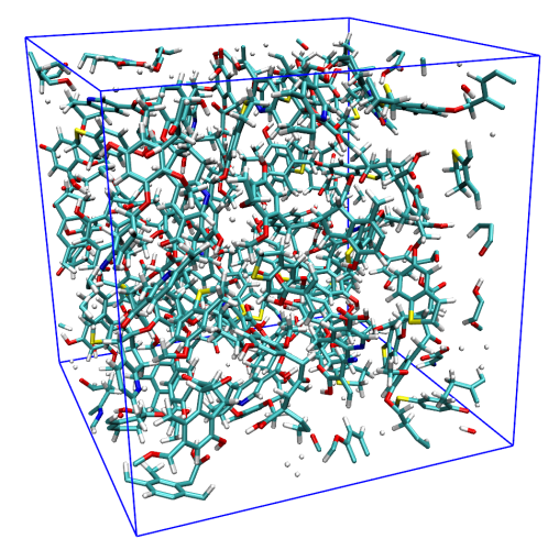
Note that if you open this file by text editor, you can find the following line:
Meaning that the box is rectangle and the length in X, Y, Z is 31.064, 31.100, 31.093 Å, respectively.
Boot up Multiwfn and input
examples\coal.pdb
300 // Other functions (Part 3)
1 // Viewing free regions and calculating free volume in a cell
4 // Set method of smoothing
1 // Gaussian function
1.8 // FWHM of Gaussian function is 1.8 times of vdW radius, which is found to be able to result in satisfactory isosurface map of smoothed grid data for present system
1 // Set grid and start calculation
[Press ENTER button] // Use default origin (0,0,0), which is suitable for present system
[Press ENTER button] // Use default box lengths, which correspond to the lengths of the three sides of the present cell
[Press ENTER button] // Use default grid space 0.25 Å, which is usually fine enough
Once the calculation of grid data is complete, you will find information about size of free regions:
Volume of entire box:   30038.649 Angstrom^3
Free volume:   14783.074 Angstrom^3, corresponding to   49.21 % of whole space
This output shows that about half of the whole cell is not lying within the vdW surface of the system.
In the newly appeared menu, select option 3 to visualize isosurface of smoothed grid data, then after selecting "Show molecule" and "Show data range" check boxes in the GUI, you will see molecular structure along with the isosurfaces representing free regions:
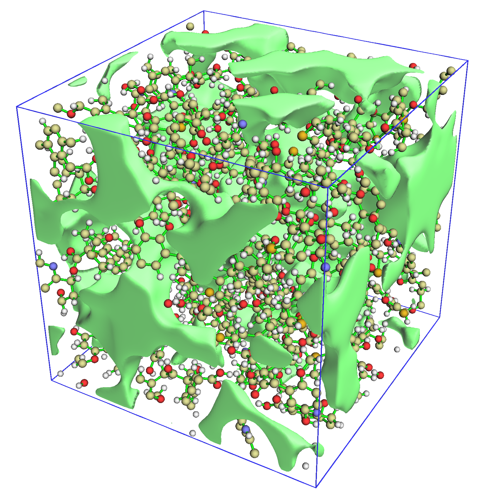
It can be seen from the map above that the actual free regions are very vividly and clearly revealed by the isosurfaces. The default isovalue is 0.5. If you increase it, the isosurfaces will shrink and only significant pores will be visible. In contrast, if you decrease isovalue, existing isosurfaces will inflate and more insignificant pores will appear in the graph.
Note
The choice of smoothing method significantly affects isosurface of smoothed grid data. As you can see from the map above, the Gaussian function with FWHM=1.8 Bohr works well for this system, but sometimes it does not work reasonably as expected. For example, when the system consists of crowded atoms (e.g. atomic clusters), this smoothing function may bring artificial effect because it decays too slowly, and sometimes the areas of the isosurfaces corresponding to free regions are too small or fully disappeared. In this case you can try other smoothing functions, such as Becke function or error function, the default one is error function with scale factor of 1.0. You can also try to Gaussian function with smaller FWHM than the present example.
In the post-processing menu, you can also export smoothed grid data as a .cub file, so that you can render it via third-part visualization tools, such as VMD, ChimeraX and VESTA. You can also find option used to visualize isosurface of raw grid data, however, as you will see, this isosurface can hardly be used to exhibit pore character in the present system, and the isosurface is very jagged, rendering importance of the smoothing algorithm employed in Multiwfn, see Section 3.300.1 for detail of the grid data calculation algorithm.
It is worth to note that as shown in Section 4.200.14.2, domain analysis module of Multiwfn is also able to visualize cavity and calculate cavity volume, however this module is only suitable for investigating internal cavity of a single molecule, it cannot be used to study all pores in a large cell like the present system.
Part 2: Covalent organic frame crystal
Multiwfn is also able to view free region and calculate its volume for experimentally determined molecular crystal. In this example I illustrate this point by taking a covalent organic frame (COF) system as an instance. Note that though the cell of this crystal is non-orthogonal, Multiwfn also works correctly.
Boot up Multiwfn and input
examples\COF_12000N2.cif
300 // Other functions (Part 3)
1 // Viewing free regions and calculating free volume in a cell
1 // Set grid and start calculation
[Press ENTER button] // Use default origin (0,0,0)
[Press ENTER button] // Use default box lengths
[Press ENTER button] // Use default grid space 0.25 Å
The quantitative data shown on screen is
Volume of entire box:    2996.151 Angstrom^3
Free volume:    1953.217 Angstrom^3, corresponding to   65.19 % of whole space
Clearly, the COF must have low density since its free volume occupies approximately as large as 2/3 of the whole cell.
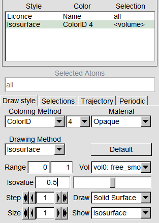
When grid is non-orthogonal, Multiwfn is unable to directly plot its isosurface map, so this time we choose option 4 in post-processing menu to export smoothed grid data as free_smooth.cub in current folder. After that, load it into VMD software (http://www.ks.uiuc.edu/Research/vmd/), go to “Graphics” - “Representation”, set drawing method of the system to “Licorice”, then add a representation for showing isosurface, and change the settings as the following screenshot (the VMD I am using is version 1.9.3)
Then in the console window, input pbc box to draw frame of grid data, and set background color to white, you will see
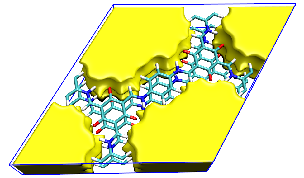
The graphical effects are very satisfactory, the free region is nicely revealed.
By the way, if you set the drawing method of the structure to “VDW”, you will find the isosurface of free region and van der Waals surface form an obvious complementarity, indicating that the free region is indeed reasonably exhibited.
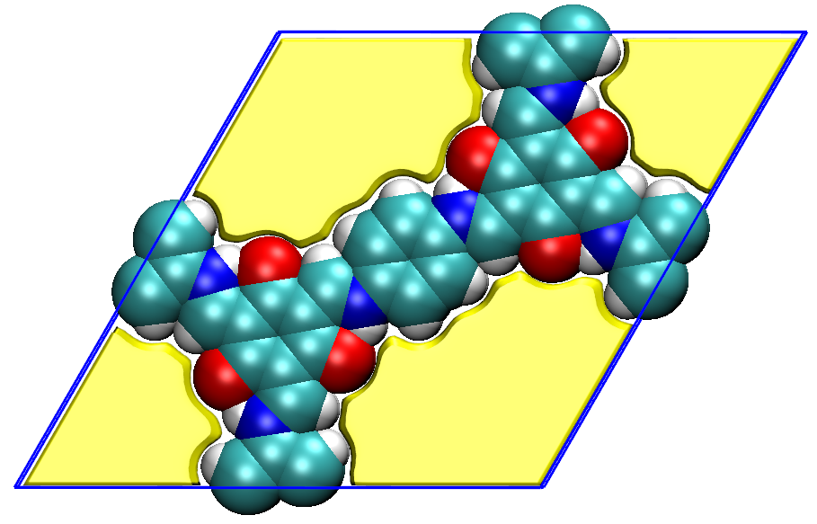
You can also use VESTA software to plot the free region map based on the free_smooth.cub, the graphical effect is even better, see http://sobereva.com/617 for detail.
4.300.2 Example of fitting radial atomic density as STOs or GTFs
Multiwfn is able to fit spherically averaged electron density of an isolated atom as multiple Slater type orbitals (STOs) or Gaussian type functions (GTFs), please read Section 3.300.2 to gain basic knowledge. In this section, I will illustrate how to use this function to realize the fitting.
4.300.2.1 Crudely fitting radial density of silicon as several STOs
In this section we will fit radial density of silicon atom as linear combination of a few STOs. Since the number of fitting functions is small, the fitting procedure is rapid and evaluation of fitted density is quite expensive, however, the fitting quality is not expected to be very high.
Boot up Multiwfn and input
examples\atomwfn\Si.wfn // Generated at ROHF/6-31G* level
300 // Other functions (Part 3)
2 // Fitting atomic radial density as multiple STOs or GTFs
3 // Check or set initial guess of coefficients and exponents of fitting functions
2 // Set initial guess as "crude fitting by a few STOs with variable exponents". Then from screen you can find only four STOs will be employed in the fitting, their initial status are
           Coefficient       Exponent
STO  1:    1.000000E+03    2.700000E+01
STO  2:    3.000000E+02    9.000000E+00
STO  3:    2.000000E+01    3.000000E+00
STO  4:    1.000000E+00    1.000000E+00
The initial parameters look reasonable. Then input below commands
0 // Return to upper level of menu
1 // Start fitting
By default, 4000 evenly distributed points with spacing of 0.001 Å are used for fitting, clearly they cover radial range of r = 0-4 Å. If you have carefully read Section 3.300.2, you will find the outputted information during the fitting is quite easy to understand. The second half of the output is shown below
Integral of fitted density calculated using 100 points:   13.13399890
Fitted coefficients are scaled by      1.06593583

Fitted parameters (a.u.) after scaling:
           Coefficient       Exponent
STO  1:   -1.995734E+00    1.190199E+00
STO  2:    2.505769E+00    1.217813E+00
STO  3:    1.004017E+02    6.877422E+00
STO  4:    2.231748E+03    3.681991E+01

RMSE of fitting error at all points:           17.562831 a.u.^2
Pearson correlation coefficient r:    0.995316  r^2:    0.990654
As you can see, the integral of the originally fitted density over the whole space is 13.13399890, therefore the coefficients of the fitting functions are scaled by 14/13.13399890=1.06593583, where 14 is the actual number of electrons of silicon. In the current fitting, both coefficients and exponents of the four STOs are optimized, the final parameters are printed under "Fitted parameters (a.u.) after scaling" title. The RMSE is a quantity useful in quantitatively measuring fitting quality. The \(r^2\) coefficient between fitted density and actual density is as high as 0.99, implying that the fitting is reasonable; however, it is highly suggested also employing other ways to further examine the fitting quality and confirm the fitting reliability, so that the fitted parameters can be safely used in practical studies to estimate density.
In the newly appeared menu you can see many options, whose meanings are either self-explanatory or have been described in Section 3.300.2.2. To quantitatively check fitting quality at the 4000 fitting points, we select option 1, then you will see
Radial distance (Angstrom), actual density (a.u.), difference between fitted an
d actual density (a.u.) as well as relative difference
#    1  r: 0.00100  rho:     1632.43875869  Diff:    548.91831985 (   33.63 %)
#    2  r: 0.00200  rho:     1580.36292117  Diff:    459.79079234 (   29.09 %)
#    3  r: 0.00300  rho:     1507.61800756  Diff:    400.75362143 (   26.58 %)
#    4  r: 0.00400  rho:     1427.66453603  Diff:    357.71394386 (   25.06 %)
[ignored...]
# 3997  r: 3.99700  rho:        0.00000506  Diff:     -0.00000029 (   -5.71 %)
# 3998  r: 3.99800  rho:        0.00000504  Diff:     -0.00000029 (   -5.81 %)
# 3999  r: 3.99900  rho:        0.00000502  Diff:     -0.00000030 (   -5.91 %)
# 4000  r: 4.00000  rho:        0.00000500  Diff:     -0.00000030 (   -6.01 %)
The "Diff" is difference between fitted density and actual density, the values in the parentheses are relative errors. As can be seen, the error in the region very close to nucleus is not small, however it does not matter since this region is not of chemical interest, usually chemists mainly focus on electron density in valence region.
Next, we choose option 3 to visually inspect curves of fitted density and actual density using logarithmic scaling, then you will see
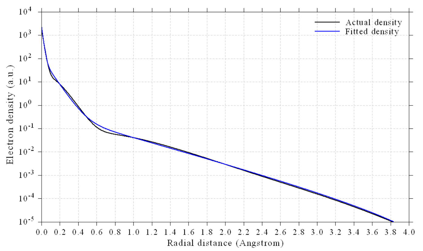
The fitting is evidently successful, since the fitted density curve is close to actual density curve in the region within 1.8 Å. It is worth to mention that Bondi vdW radius of silicon is 2.1 Å.
You can also select option 4 to plot comparison map between fitted density and actual density using linear scaling, you will further find that the fitted density indeed nicely reproduces the actual density.
If you select option 5, then fitdens.txt will be outputted in current folder. This file contains fitted density (the second column) at points evenly distributed from 0 to 10 Å, the grid spacing is half of the fitting points, namely 0.001/2=0.0005 Å. From the data in this file you can find that the fitted density varies smoothly and monotonically, no negative value can be found, further implying that the fitting is successful and the fitted parameters are reliable.
Finally, we select option 6 to examine integral of fitted density over the whole space via different number of points of Gaussian quadrature, you will see:
Number of integration points:   40    Integral:     13.99999923
Number of integration points:   60    Integral:     13.99999993
Number of integration points:   80    Integral:     13.99999999
[ignored...]
Number of integration points:  280    Integral:     14.00000000
Number of integration points:  300    Integral:     14.00000000
As can be seen, in all cases the integral is almost exactly identical to the actual number of electrons (14), further demonstrating that our fitting is reasonable.
Since our fitted density has passed quality check in many ways, we can finally conclude that the fitted parameters of the four STOs can be safely and reliably employed in future research.
4.300.2.2 Accurately fitting radial density of bromine as many GTFs
In order to reliably and exactly fit radial density, usually no less than 10 GTFs (with variable exponents) are needed. In this example we will fit radial density of bromine atom in this way. This kind of fitting is almost suitable for any element in the periodic table.
Boot up Multiwfn and input
examples\atomwfn\Br.wfn // Generated at ROHF/6-31G* level
300 // Other functions (Part 3)
2 // Fitting atomic radial density as STOs or GTFs
3 // Check or set initial guess of coefficients and exponents of fitting functions
5 // Fine fitting by 10 GTFs with variable exponents (of course, using more GTFs will result in better fitting)
As can be seen from screen, 10 GTFs will be employed in the fitting, all coefficients are initially set to 1.0, while their exponents span large range, the smallest one is 0.1, while the largest one is 381, the ratio between two neighbouring GTFs is 2.5. The GTFs with small, medium and large exponents are mainly used to represent tail region, valence region and the region very close to nucleus, respectively.
Then input 0 to return to upper level of menu and then choose option 1 to start fitting. During fitting, from prompt you can find 1 redundant fitting function is automatically eliminated to avoid numerical problems, which has a very small coefficient:
Delete redundant function (coeff=-5.59231E-05 exp= 9.99991E-02), refitting...
Totally  1 redundant fitting functions have been eliminated
The resulting fitted parameters:
Fitted parameters (a.u.) after scaling:
           Coefficient       Exponent
GTF  1:    8.328778E-02    2.556435E-01
GTF  2:    5.163781E-01    6.322086E-01
GTF  3:    1.221206E+01    5.157472E+00
GTF  4:    2.475569E+01    5.176644E+00
GTF  5:    5.926930E+02    6.326802E+01
GTF  6:    4.017684E+03    7.298312E+02
GTF  7:    1.006232E+04    2.458635E+03
GTF  8:    1.046461E+04    1.557579E+04
GTF  9:    1.658191E+07    1.206884E+09
and you can find error statistics:
From this data we can find the fitting quality is almost perfect! The \(r^2\) is almost exactly 1.0!
Please use the same way as illustrated in the last section to examine fitting quality, you will find current fitting is completely successful. For example, after choosing option 3 we can see the following map, which exhibits that the fitting quality in all regions is perfect.
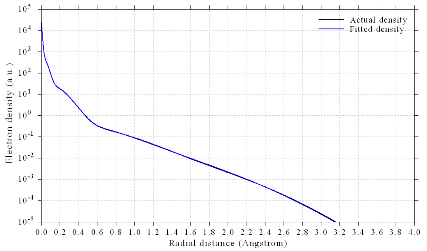
Clearly, the fitting procedure illustrated in this section is quite ideal when you want to reach very high fitting quality.
By the way, from the parameters of the fitted GTF functions shown earlier, you can find GTF 3 and GTF 4 have almost identical exponent, that means they can be combined as a single GTF to reduce the parameters. To do so, we input
0 // Return
3 // Check or set initial guess of coefficients and exponents. Then from screen you can find the parameters we fitted earlier
10 // Combine two fitting functions together
3,4 //Indices of the two fitting functions to combine
0 // Return
1 // Start fitting
Then you can use option 3 to visualize the radial density again, you will find the quality of the fitting via the current 8 GTFs is unchanged, so 8 GTFs are fully adequate to reach an accurate fitting for present atom.
The fitting module in Multiwfn is quite flexible, there are many options used to control fitting strategy, see Section 3.300.2 for more information.
4.300.4 Example of simulating scanning tunneling microscope (STM) image
Note
Chinese version of this topic is my blog article “Using Multiwfn to simulate scanning tunneling microscopy (STM) images” (http://sobereva.com/549, in Chinese), in which extended discussion is given and cyclo[18]carbon is taken as example.
Please check Section 3.300.4 if you are not familiar with theory of STM or simulation of STM in Multiwfn. In the next two sections, we will respectively simulate STM of constant height and constant current modes for phenanthrene. The simulation will be based on the wavefunction in examples\phenanthrene.fch, which was generated at B3LYP/6-31G* level.
It is important to note that in order to simulate STM in Multiwfn, the molecule must be parallel to XY plane (though the molecule is not necessarily planar), however, in the phenanthrene.fch the molecule is parallel to YZ plane. Therefore, the molecule must be rotated prior to STM simulation. Of course, we can first reorient the molecule and then conduct a single point task via quantum chemistry to generate wavefunction file, but a better way is using Multiwfn to directly rotate the wavefunction and geometry, namely inputting below commands in Multiwfn
examples\phenanthrene.fch
6 // Check & modify wavefunction
33 // Rotate wavefunction, namely X→Y, Y→Z, Z→X
0 // Rotate all orbitals
y // Also rotate molecule structure. Then the molecule will be on XZ plane
33 // Rotate wavefunction again
0 // Rotate all orbitals
y // Also rotate molecule structure
Now the phenanthrene has exactly been on XY plane of Z=0 Å (you can check this point via main function 0). Then we enter main function 100, choose subfunction 2 and then select corresponding option to export the present wavefunction to a new .mwfn file. In the next sections, this new file will be referred to as mol.mwfn.
4.300.4.1 Simulating constant height STM image for phenanthrene
Here we simulate STM image of constant height mode for phenanthrene. Boot up Multiwfn and input
mol.mwfn
300 // Other function (Part 3)
4 // Simulating STM image
From the message on screen, it can be seen that the Fermi level (\(E_{\mathrm{F}}\)) has been set to average of HOMO energy and LUMO energy, the bias voltage (V) has been automatically set to the difference between HOMO energy and \(E_{\mathrm{F}}\), in this case only HOMO can contribute to the STM image. In order to obtain expected STM image, it is crucial to properly define the V. In the case of negative V, electrons flow from sample to STM tip, and the more negative the V, the more MOs may contribute to the STM image. Also, note that the distance between the atoms in the sample and the tip significantly affects STM image. From the information on option 7 you can find the default Z coordinate of the plane to be plotted is 0.7 Å. Since all atoms in the mol.mwfn have Z coordinate of 0 Å, the distance between the nuclei and the tip is 0.7 − 0.0 = 0.7 Å. In this example, we will plot STM image with V= -5.0 V at Z=1.2 Å.
Now input below command
2 // Set bias voltage
-5 // Bias voltage of -5.0 V
7 // Set Z coordinate
1.2 // Z=1.2 Å
0 // Calculate tunneling current on the plane
Now you can find the information below on screen
Lower limit of MO energy considered in the calculation:      -8.362 eV
Upper limit of MO energy considered in the calculation:      -3.362 eV
The MOs taken into account in the current STM simulation:
MO    44   Occ= 2.000   Energy=     -7.6491 eV   Type: Alpha&Beta
MO    45   Occ= 2.000   Energy=     -7.0599 eV   Type: Alpha&Beta
MO    46   Occ= 2.000   Energy=     -6.0337 eV   Type: Alpha&Beta
MO    47   Occ= 2.000   Energy=     -5.7308 eV   Type: Alpha&Beta
Totally   4 MOs are taken into account

Grid spacings in X and Y are    0.118428    0.082980 Bohr
Calculating, please wait...
Maximal value (LDOS) is    0.010218 a.u.
It can be seen that there are 4 occupied MOs whose energy is lying between \(E_{\mathrm{F}}\)+eV (-8.362 eV) and \(E_{\mathrm{F}}\) (-3.362 eV), therefore the plane data of the STM image corresponds to sum of their probability densities in the plane multiplied by their occupation numbers (2.0 in present case since they are all close-shell MOs), this data is also known as local density-of-states (LDOS). As shown in the prompt, the largest value of LDOS in the calculated plane is 0.010218 a.u.
Now you are in the STM plotting menu, you can find many options used to adjust plotting effect, they are all self-explanatory, please play with them. We directly choose option 0 to plot the image under default setting, you will see
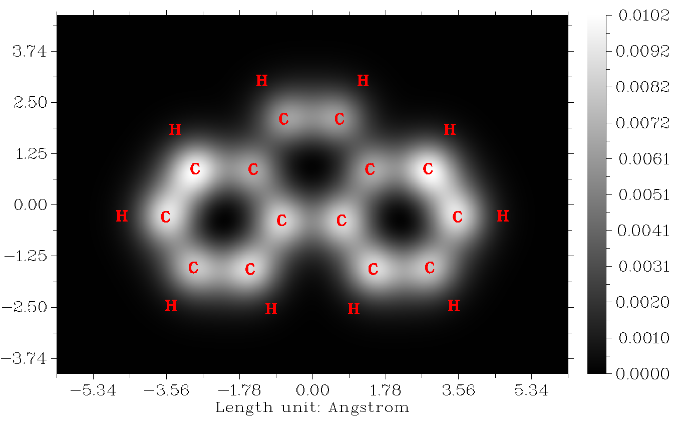
In this map, the brighter the white, the larger the LDOS and thus the stronger the tunneling current (I), since the Tersoff-Hamann model shows that I is positively proportional to LDOS. It can be seen that I signal is more prominent over the two boundary six-membered rings than the central one.
4.300.4.2 Simulating constant current STM image for phenanthrene
In this section we again plot STM image for phenanthrene but using constant current mode. Boot up Multiwfn and input
mol.mwfn
300 // Other function (Part 3)
4 // Simulating STM image
1 // Switch the mode of STM image to constant current
2 // Set bias voltage
-5 // Again we use bias voltage of -5.0 V
In the constant current mode, LDOS is calculated for every evenly distributed point in a 3D region, whose X, Y and Z range can be set by options 5, 6 and 7, respectively, usually the default setting is appropriate. We directly choose option 0 to start the calculation, from the information on screen you can find the maximal value of LDOS in the calculated region is 0.048 a.u.
In the post-processing menu, you can find several options, we first use option 1 to visualize isosurface map of tunneling current, which corresponds to LDOS in the present context. The isosurface corresponding to LDOS=0.015 a.u. is shown below. Note that although the choice of isovalue is arbitrary, it should be between 0 and the maximum value (0.048 a.u. in this example)
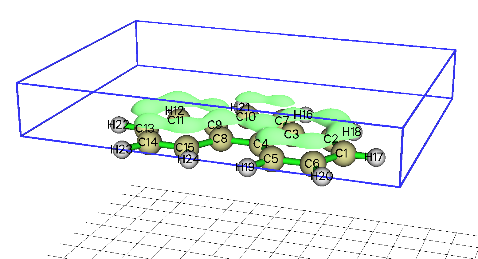
In the map above, the isosurfaces of tunneling current normally occur over the carbons, implying that the default calculated region is appropriate for the present case. The blue box can be shown by clicking "Show data range" check box, it displays the region where LDOS was calculated.
Next, we plot plane map. Select option "3 Calculate and visualize constant current STM image" and then input the expected value of tunneling current, we input 0.01 in this example. After that, Multiwfn starts to calculate the Z value where tunneling current (LDOS) is approximately equal to 0.01 a.u., evidently Z is different at different (x,y) positions. Then from screen you can find
They are proper lower and upper limits of the color scale of STM image, respectively.
Now you are in the interface of plotting STM image of constant current mode, we input below commands
2 // Choose map type
2 // Color-filled map with contour lines
7 // Set label interval in X, Y and color scale axes
1.5,1.5,0.05
-3 // Change other plotting settings
2 // Set number of decimal places of tick labels
1 // Set X axis
1 // Set Y axis
2 // Set Z axis
0 // Return
0 // Plot the STM image
Then you can see this map on screen:
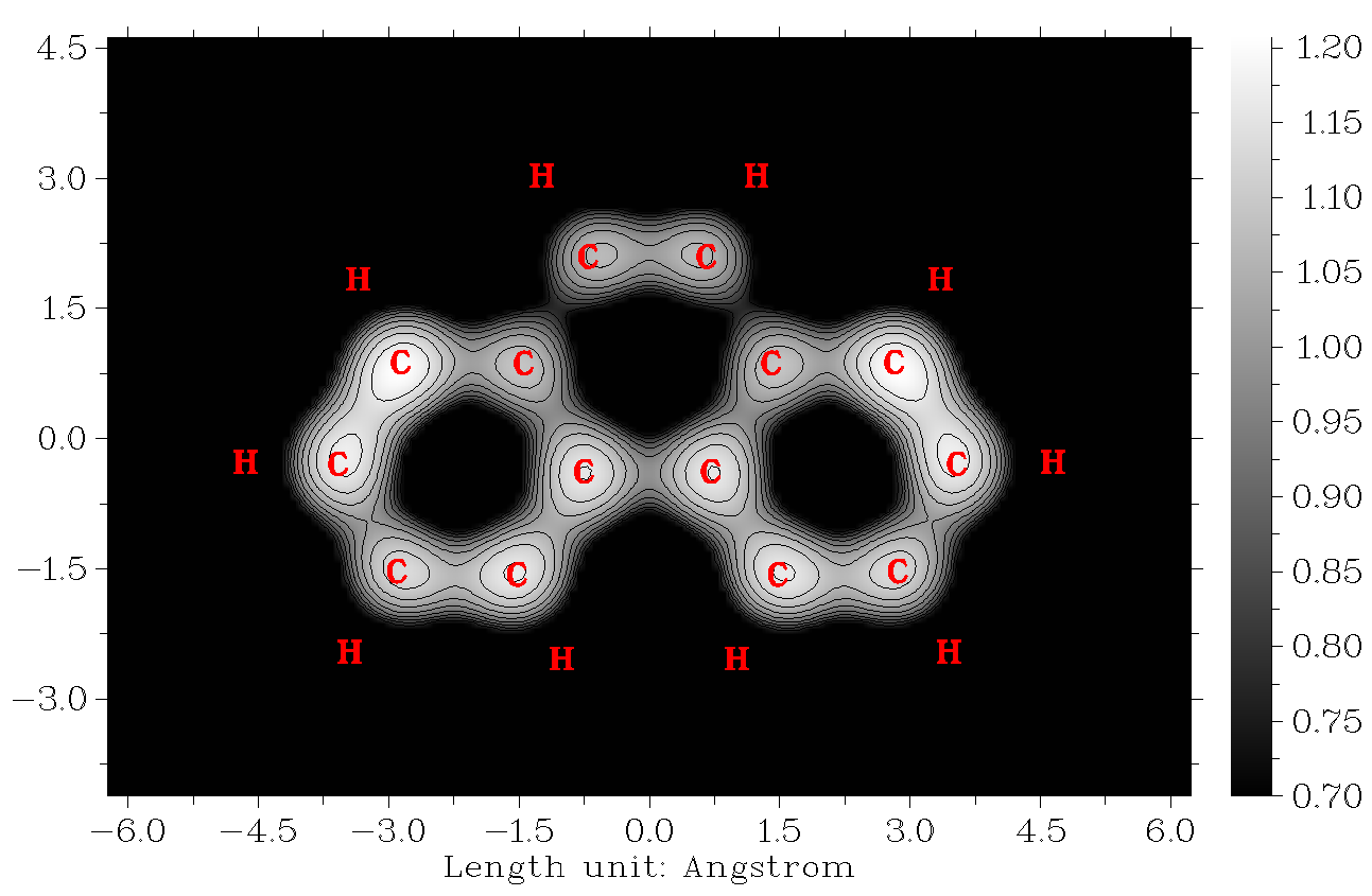
In the map above, the value corresponds to Z distance of STM tip. It can be seen that at constant current (LDOS) of 0.01 a.u., the Z position of STM tip is relatively high over the two boundary six-membered rings. The characteristic of this map is very similar to the STM image of constant height mode.
If you want to further investigate the STM plane map with other constant current values, you can exit the plotting interface, then enter the option "3 Calculate and visualize constant current STM image" again and input the expected current value.
4.300.5 Calculate electric dipole moment, multipole moments and electronic spatial extent for uracil
As described in Section 3.300.5, Multiwfn is able to analytically calculate electric dipole moment, quadrupole, octopole, hexadecapole moments and electronic spatial extent <\(r^2\)>. In this section we calculate these quantities for a simple molecule, uracil.
Boot up Multiwfn and input
examples\uracil.wfn
300 // Other function (Part 3)
5 // Calculate electric dipole moment and multipole moments
The calculation is quite fast, you will immediately see the following information, which is very easy to understand if you have read Section 3.300.5. As clearly indicated on screen, the unit is a.u. unless otherwise specified.
 Dipole moment from nuclear charges (a.u.):    0.000000   0.000000   0.000000
 Dipole moment from electrons (a.u.):          0.473309   1.823683   0.000736

 Dipole moment (a.u.):       0.473309      1.823683      0.000736
 Dipole moment (Debye):      1.203031      4.635340      0.001872
 Magnitude of dipole moment:      1.884103 a.u.      4.788911 Debye

 Quadrupole moments (Standard Cartesian form):
 XX=  -43.878975  XY=    1.812455  XZ=   -0.000544
 YX=    1.812455  YY=  -28.230039  YZ=   -0.004831
 ZX=   -0.000544  ZY=   -0.004831  ZZ=  -34.463441
 Quadrupole moments (Traceless Cartesian form):
 XX=  -12.532235  XY=    2.718682  XZ=   -0.000816
 YX=    2.718682  YY=   10.941169  YZ=   -0.007246
 ZX=   -0.000816  ZY=   -0.007246  ZZ=    1.591066
 Magnitude of the traceless quadrupole moment tensor:   13.645453
 Quadrupole moments (Spherical harmonic form):
 Q_2,0 =   1.591066   Q_2,-1=  -0.008367   Q_2,1=  -0.000942
 Q_2,-2=   3.139264   Q_2,2 = -13.552376
 Magnitude: |Q_2|=   14.001908

 Octopole moments (Cartesian form):
 XXX=   14.0946  YYY=    8.6123  ZZZ=    0.0027  XYY=    6.6643  XXY=   46.4098
 XXZ=   -0.0099  XZZ=    2.7809  YZZ=   -7.6843  YYZ=    0.0159  XYZ=   -0.0033
 Octopole moments (Spherical harmonic form):
 Q_3,0 =    -0.0062  Q_3,-1=   -52.5167  Q_3,1 =    -5.9005
 Q_3,-2=    -0.0129  Q_3,2 =    -0.0500  Q_3,-3=   103.2618  Q_3,3 =    -4.6630
 Magnitude: |Q_3|=    116.0929

Hexadecapole moments:
XXXX=       -684.9560  YYYY=       -289.5418  ZZZZ=        -39.7011
XXXY=         13.4854  XXXZ=         -0.0058  YYYX=         12.7574
YYYZ=         -0.0243  ZZZX=         -0.0009  ZZZY=         -0.0061
XXYY=       -168.4269  XXZZ=       -104.4367  YYZZ=        -71.1599
XXYZ=         -0.0008  YYXZ=         -0.0039  ZZXY=          2.9446

Electronic spatial extent <r^2>:      822.650952
Components of <r^2>:  X=     501.328431  Y=     286.859071  Z=      34.463450
If "ispecial" in settings.ini is set to 1, then before calculating dipole and multiple moments, the system will be displaced to make nuclear contribution to dipole moment zero.
Note that you can also use subfunction 2 of main function 15 to calculate above quantities, however it calculates numerically based on multicenter grids, the cost is significantly higher while the numerical accuracy is slightly lower. However, it has a unique advantage, namely it can calculate dipole and multipole moments for specific fragments in current system, see Section 4.15.3 for example.
The <\(r^2\)> is a useful index to quantitatively characterize the breadth of the distribution of electrons, I have a blog article to discuss this point in detail: http://sobereva.com/616 (in Chinese).
4.300.6 Calculating orbital energies: NTO orbital as an example
As described in Section 3.300.6, Multiwfn has a function to evaluate energies of the orbitals stored in memory based on the user-provided Fock/Kohn-Sham matrix. In principle, one can use this function to calculate energies of orbitals of any kind! In this example, I will illustrate how to make use of this function to evaluate energies of natural transition orbitals (NTOs). S0→S1 excitation of a typical donor-π-acceptor system will take as the example. Please make sure that you have understood how to perform NTO analysis, see Section 4.18.6 for example. The present example contains three steps: (1) Generating NTO orbitals by TDDFT calculation (2) Generating a file containing Fock/Kohn-Sham matrix (3) Calculating NTO orbital energies.
First, we generate NTO orbitals, the Gaussian input file of TDDFT task is examples\excit\D-pi-A.gjf, the corresponding output file and .fchk file have also been provided in the same folder. Boot up Multiwfn and input the following commands
examples\excit\D-pi-A.fchk
18 // Electron excitation analysis
6 // Generate natural transition orbitals (NTOs)
examples\excit\D-pi-A.out
1 // The first excited state (S1 state)
Then you can see
The highest 10 eigenvalues of occupied NTOs:
   0.000022    0.000023    0.000038    0.000057    0.000105
   0.000149    0.000172    0.000339    0.008236    0.992492

The highest 10 eigenvalues of virtual NTOs:
   0.992492    0.008236    0.000339    0.000172    0.000149
   0.000105    0.000057    0.000038    0.000023    0.000022
These data display that NTO works well for the present case, since the NTO pair with highest eigenvalue contributes 99.2% to this excitation, namely the S0→S1 excitation can be almost perfectly represented by this NTO transition. Then we choose option 3 to export the NTOs as NTO.mwfn in current folder.
Next, we generate a file containing Kohn-Sham matrix of present system, see Section 3.100.17 for details. Boot up Multiwfn and input
examples\excit\D-pi-A.fchk
100 // Other functions (Part 1)
17 // Generate Fock/KS matrix based on orbital energies and coefficients
KS.txt
Now the KS.txt in current folder contains the Kohn-Sham matrix converted back from the energies and coefficients of molecular orbitals in the D-pi-A.fchk.
Finally, we calculate energies of the NTO orbitals. Boot up Multiwfn and input
NTO.mwfn
300 // Other functions (Part 3)
6 // Calculate energies of the present orbitals
KS.txt
Then Multiwfn loads Kohn-Sham matrix from the KS.txt file, and the calculation of the NTO orbital energies is finished immediately. You can then export the energies to orbene.txt in current folder by choosing “1 Export orbital energies to orbene.txt in current folder”, the content will be
[...ignored]
     54  Occ=  2.0000  E=     -0.41616309 Hartree    -11.3244 eV
     55  Occ=  2.0000  E=     -0.27176663 Hartree     -7.3951 eV
     56  Occ=  2.0000  E=     -0.34791315 Hartree     -9.4672 eV
     57  Occ=  0.0000  E=     -0.02609500 Hartree     -0.7101 eV
     58  Occ=  0.0000  E=      0.03073422 Hartree      0.8363 eV
     59  Occ=  0.0000  E=      0.76811627 Hartree     20.9015 eV
[...ignored]
In the NTO.mwfn, the occupied and unoccupied NTOs with highest eigenvalue are orbitals 56 and 57, respectively, according to the above data their energies are found to be -9.4672 and -0.7101 eV, which are very reasonable.
Note that there are also other ways to provide Kohn-Sham matrix to Multiwfn, see Appendix 7 of this manual. For example, you can also use Gaussian to directly generate .47 file, which can also provide Kohn-Sham matrix to Multiwfn for generating orbital energies. Now I illustrate how to do. We create a new Gaussian input file with the following content, notice that the geometry, DFT functional and basis set must be exactly identical to the examples\excit\D-pi-A.gjf. (this file has already been provided as examples\excit\D-pi-A_get47.gjf)
# CAM-B3LYP/6-31g(d) pop=nboread

b3lyp/6-31g(d) opted

0 1
[geometry part]

$NBO archive file=C:\D-PI-A $END
After running this file by Gaussian, you will obtain D-PI-A.47 file in C: folder, it has been provided as examples\excit\D-PI-A.47. Then after choosing subfunction 6 in main function 300, you can input path of this .47 file, Multiwfn will load Kohn-Sham matrix from it and then calculate orbital energies.
Note
Due to numerical reasons, the Kohn-Sham matrix recorded in the .47 file and that directly generated by Multiwfn are marginally different, hence the resulting NTO energies are also slightly different in the two cases. However, the difference is fully negligible for practical studies.
When diffuse functions are heavily employed and thus quantum chemistry code automatically eliminated some linearly dependent basis functions, Multiwfn will be unable to directly generate Kohn-Sham matrix, and you have to use other ways to provide Kohn-Sham matrix to Multiwfn, such as using .47 file.
4.300.8 Plotting surface distance projection map for [Ru(bpy)3]2+ cation coordinate
Note
Chinese version of this tutorial with more discussions is "Using Multiwfn to plot surface distance projection map for molecules and solids" (http://sobereva.com/589).
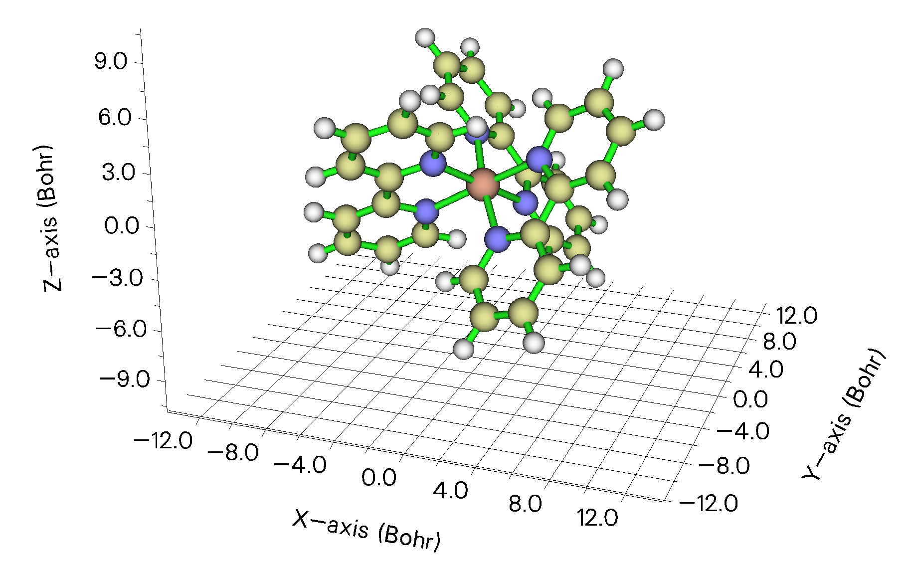
Please read Section 3.300.8 first to gain basic knowledge about the molecular surface distance projection map. In this section, [Ru(bpy)3]2+ will be taken as an example to show how to plot this kind of map. The examples\excit\Ru(bpy3)2+.gjf contains optimized geometry of this system, therefore it will be used as input file (of course, you can also use file in other formats such as .xyz, .pdb and .mol2 as input file). The system is already in an appropriate orientation for studying burying of Ru atom by the ligands, see below figure. If the current orientation is not suitable for plotting this map, you should use molecular visualization softwares such as GaussView to rotate it.
Boot up Multiwfn and input
examples\excit\Ru(bpy3)2+.gjf
300 // Other functions (Part 3)
8 // Plot molecular surface distance projection map
This time we do not alter any default setting, but simply select option 0 to start calculation. In this case, the molecular surface is defined as isosurface of promolecular electron density of 0.05 a.u.
Once the calculation is finished, you will enter an interface for plotting plane map. We directly choose option 0 to show the map on screen, you will see
![Surface distance projection map of the [Ru(bpy)3]2+ cation](../assets/figures/ch4/image1432.png)
As you can see, different colors nicely exhibit the distance of various regions of molecular surface to screen, the relative position of Ru atom and ligands can be very clearly detected. Under the default setting, Z=0 corresponds to the Z position of the atom having most positive Z coordinate. If the current map does not make you satisfied, you can close the map and use the rich options in the interface to further improve graphical effect.
Next, we plot this map again but using another molecular surface definition, namely superposition of atomic van der Waals spheres. Now input the following commands
-1 // Return
1 // Set definition of molecular surface
3 // Superposition of atomic van der Waals spheres scaled by a factor
1 // We do not scale van der Waals radii in this example, so we set scale factor to 1
0 // Start calculation
0 // Show the map on screen
Then you will see the following figure, from which it is obvious that the Ru atom is heavily buried by surrounding ligands, and due to the strong steric hindrance, foreign molecules are not easy to approach the Ru atom.
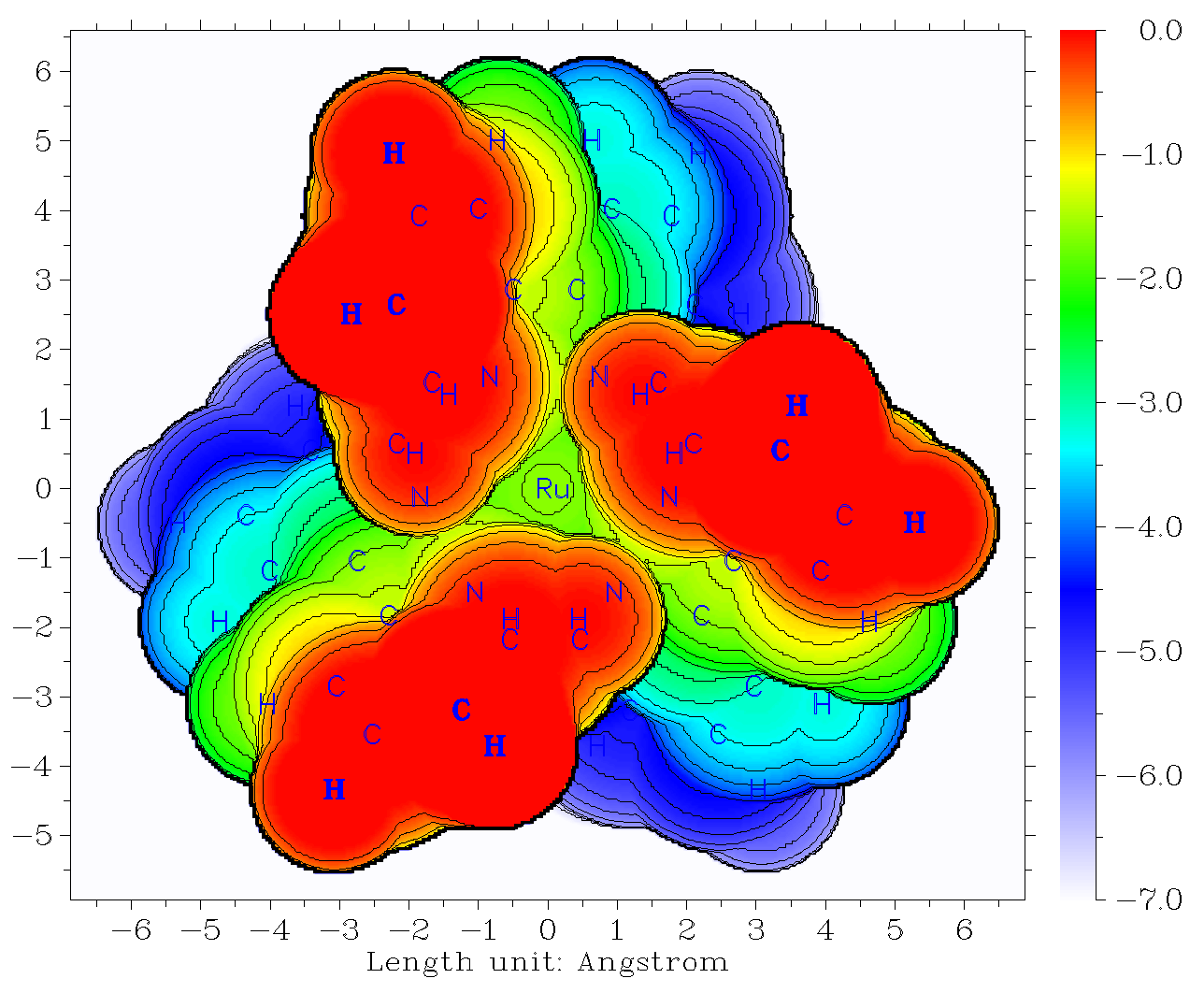
The van der Waals surface constructed by superposition of atomic spheres is evidently not quite smooth. Using 0.005 a.u. of electron density isosurface as definition of molecular surface can produce a map with comparable character, while the color transition and contour lines are much smoother (after returning to last menu, you can choose option 1, select 1 and then input 0.005 to switch to this definition).
Note that Multiwfn is also able to plot this kind of map for solid surface, see Section 4 of http://sobereva.com/589 for illustration.