4.19 Orbital localization analysis

Note

Most information in this section is also available in my blog article “The use of orbital localization function of Multiwfn and its comparison with NBO and AdNDP analyses” (http://sobereva.com/380, in Chinese).

Orbital localization is a very powerful and useful technique, it can transform canonical molecular orbitals, which often show highly delocalized character, to localized form, which is known as localized molecular orbital (LMO). The LMOs have close relationship with many classical chemistry concepts such as chemical bond and lone pair, therefore they can be used to analyze and unveil many problems of chemical interest. Before reading this section, please read Section 3.22 first to gain some basic knowledge. Some examples in other sections, such as the example in Sections 4.8.4 and 4.100.22, also utilized orbital localization function.

CAUTION: The default orbital localization method, namely Pipek-Mezey based on Mulliken population (PM-Mulliken) method is not suggested to use when diffuse functions are heavily employed, otherwise the result may be misleading. If diffuse functions have to be employed, you should change to Pipek-Mezey based on Becke population (PM-Becke) method, or Foster-Boys method, see Section 3.22 for introduction of pros and cons of various orbital localization methods.

4.19.1 Localizing molecular orbital of 1,3-butadiene by Pipek-Mezey method

This section illustrates the use of orbital localization analysis of Multiwfn with trans-1,3-butadiene as example.

Basic steps of performing LMO analysis

The input file is examples\butadiene.fch, which was yielded at B3LYP/6-31G** level. You can first visualize its MOs via main function 0, you will find all MOs are highly delocalized, none of them have direct correlation with classical concept of chemical bond theory. Now we perform orbital localization to transform them into more chemically meaningful orbitals. Boot up Multiwfn and input

examples\butadiene.fch
19  // Orbital localization. By default, Pipek-Mezey localization method based on Mulliken population is used
2  // Perform localization for both occupied and unoccupied MOs

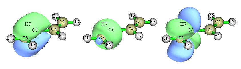
Since this system is small, convergence of localization iteration immediately achieved, and the major character of the resulting orbitals are printed. After that Multiwfn automatically exports the LMOs as new.fch in current folder and then loads it. Now, the orbital coefficients in memory have been completely updated to the LMOs. You can use different ways to characterize them. We enter main function 0 to visualize these orbitals, you will find all orbitals show strong localization character, in particular the occupied ones. Below are screenshots of three LMOs involving C6-C8, the first two are occupied, and they correspond to σ bond and π bond, respectively; the third one is unoccupied, it can be ambiguously identified as anti-π bond orbital.

Evaluating LMO energies

It is possible to evaluate energies for the LMOs, as illustrated below. Boot Multiwfn and input

examples\butadiene.fch
19  // Orbital localization
-4  // Allow Multiwfn to generate and print energy for LMOs
1  // Evaluate energies of the LMOs using the Fock matrix generated by MO energies and coefficients via F=SCEC^-1 relationship
2  // Localize both occupied and unoccupied orbitals

After calculation is finished, Multiwfn evaluates energies of the LMOs and sort them according to their energies from low to high. You can find energies of all LMOs from screen. The information of the highest occupied and lowest unoccupied LMOs is shown below

   14   Energy:   -0.2750728 a.u.      -7.4851 eV   Type: A+B   Occ: 2.0
   15   Energy:   -0.2750728 a.u.      -7.4851 eV   Type: A+B   Occ: 2.0
   16   Energy:    0.2185911 a.u.       5.9482 eV   Type: A+B   Occ: 0.0
   17   Energy:    0.2185913 a.u.       5.9482 eV   Type: A+B   Occ: 0.0

Please plot these orbitals in main function 0 to try to identify their characters.

Note

By the way, it is also possible to evaluate energies of the LMOs based on the Fock matrix loaded from an external file (see Appendix 7 for details), and this is the only choice if the Fock matrix cannot be successfully generated based on MO energies and coefficients. For example, the Fock matrix can be loaded from NBO .47 file; to realize this for present system, we can enter main function 100 and choose subfunction 2, and then select option 10 to export current system as a Gaussian input file. Then properly modify the input file to request Gaussian to output .47 file, and we need to ensure that the calculation level is identical to the examples\butadiene.fch (B3LYP/6-31G**). The prepared input file has been provided as examples\butadiene_47.gjf. Run it by Gaussian, you will find the resulting BUTADIENE.47 at C: (this file has already been provided as examples\butadiene.47). In the main function 19, after choosing option -4 to allow Multiwfn to evaluate LMO energies, if you select suboption “2 Evaluate, loading Fock matrix from a file” and then input the path of the .47 file, the Fock matrix recorded in the .47 file will be loaded and will be used to evaluate the LMO orbital energies in due time

Showing center positions of all LMOs

It is possible to visualize center positions of all generated LMOs, so that the distribution of the LMOs can be immediately understood. Here I illustrate how to realize this.

Reboot Multiwfn and input

examples\butadiene.fch
19  // Orbital localization
-8  // Switch status of “If calculating center position and dipole moment of LMOs” to “Yes”
-6  // Change localization method
10  // Foster-Boys
1  // Localize occupied orbitals (center position of unoccupied LMOs is generally uninteresting therefore we do not localize unoccupied MOs)
n  // Skip the dipole moment analysis

As you can see from the prompts, after orbital localization has been finished as usual and the newly generated new.fch has been automatically loaded into Multiwfn, the program calculates center position of each LMO. In order to make visualization of the centers easy, Multiwfn adds Bq atoms (i.e. ghost atoms”) into the current system to represent the centers of the LMOs. The center coordinates as well as correspondence between LMO indices and Bq indices are automatically exported to current folder as LMOcen.txt. The content of this file of current instance is

 LMO     1 corresponds to Bq    11, X,Y,Z:    1.1372    0.7759   -0.0000 Bohr
 LMO     2 corresponds to Bq    12, X,Y,Z:   -1.1372   -0.7759   -0.0000 Bohr
 LMO     3 corresponds to Bq    13, X,Y,Z:    1.1372    3.3081   -0.0000 Bohr
...[ignored]

Then we return to main menu and enter main function 0 to visualize the LMO centers and orbital isosurfaces. The plotting settings have been automatically set to a special status for best visualizing LMOs purpose, currently you can see:

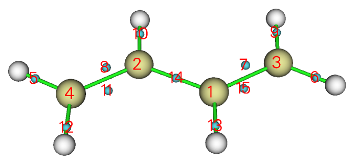
From this graph we can very clearly understand distribution of the generated LMOs. Each cyan sphere is a ghost atom, representing center of a LMO. Under current setting the index of the ghost atoms starts from 1, therefore the index shown in the graph directly corresponds to the LMO index. For example, we want to simultaneously visualize the two LMOs at boundary C-C bond, since the cyan spheres with labels 8 and 11 locate around the bond, we choose orbital 8 in the orbital list to display it, then select “Show+Sel. isour#2” and choose orbital 11 to. After that, change isovalue to 0.13 and set the drawing style as transparent, you will see

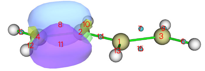
Evidently, the two LMOs obtained via Foster-Boys method collectively represent the double-bond character of the boundary C-C bond. The two LMOs are known as “banana” orbitals and do not exhibit σ-π separation character.

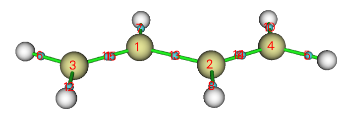
You can also try to visualize the center position of the LMOs generated via Pipek-Mezey algorithm. Because this method represents each double-bond as a pair of separated σ and β LMOs, whose centers should be very close to each other, from the graph below you can find the centers indeed can hardly be distinguished:

It is worth to note that there are two ways to rapidly find the index of the LMO corresponding to the bond of your interest. The first one is examining the orbital compositions printed during the orbital localization, the second one is directly visualizing the LMO centers and finding the index showing above the cyan sphere at proper place, as I just illustrated.

4.19.2 Analyze variation of localized molecular orbitals for SN2 reaction

In this example, we study variation of localized molecular orbitals (LMOs) along with reaction path to visualize variation of chemical bonds, a typical SN2 reaction is taken as instance.

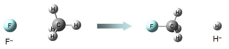
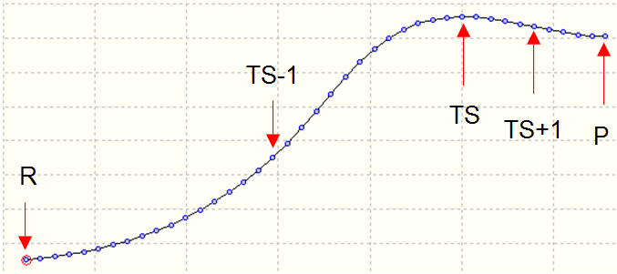
This SN₂ reaction involves formation of F-C bond and break of C-H bond, therefore in the following analysis we will focus on corresponding two LMOs. The IRC of the SN₂ reaction is shown below, five points are taken into account, their .fch files have been provided in examples\SN2 folder.

First, we generate LMOs for transition state (TS) geometry. Boot up Multiwfn and input

examples\SN2\TS.fch
19  // Orbital localization
1  // Localize occupied orbitals
0  // Visualize orbitals

We can find there are two orbitals respectively corresponding to F-C and C-H bonds, we draw them together for easier comparison

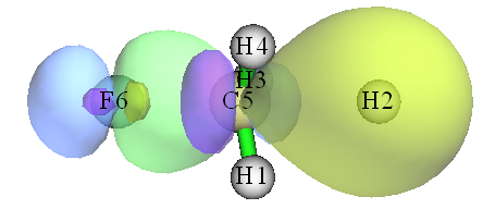
The green-blue isosurface and purple-yellow isosurfaces clearly portray the orbitals corresponding to F-C and C-H bonds, respectively.

We draw the same kind of plot for R.fch, TS-1.fch, TS+1.fch and P.fch, then put the graph together, as shown below

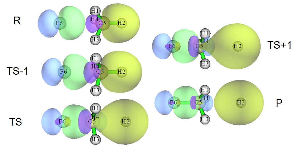
From the graph, the variation of chemical bonds during the SN₂ reaction is quite clear (R→TS-1→TS→TS+1→P). In the reactant state, the green-blue isosurface corresponds to the lone pair of the fluorine atom, while the purple-yellow isosurface shows typical covalent bond character of C-H. As the reaction proceeds, the two LMOs vary smoothly, the C-F covalent bond character becomes more and more prominent, and in the final product state, the LMO represented by purple-yellow isosurface has already corresponded to 1s orbital of H^- anion.

4.19.3 Characterize Re-Re bond of [Re₂Cl₈]^2- anion

It is widely accepted that the Re-Re bond in [Re₂Cl₈]^2- anion is a quadruple bond, with configuration of (σ²π⁴δ²). The σ bond results from overlap of \({d}_{{z}^{2}-{p}_{z}}\) hybrid orbitals of the two rhenium atoms, the two π bonds stem from overlap of their \(d_{\mathrm{xz}}\) and \(d_{\mathrm{yz}}\) orbitals, while the δ bond is formed by overlap of their \(d_{\mathrm{xy}}\) orbitals. Can this classic concept be validated via orbital localization analysis?

The .fchk file of [Re₂Cl₈]^2- anion produced under B3LYP with 6-31G* for Cl and SDD for Re is provided as examples\Re2Cl82-.fchk. Load it into Multiwfn and carry out orbital localization for occupied orbitals, from the output we can immediately identify the four LMOs corresponding to the Re-Re bond:

Hint

If you want to more easily find the indices of the LMOs corresponding to the Re1-Re2 bond, the best way is setting "iprintLMOorder" in settings.ini to 1 before booting up Multiwfn. After that, the compositions of LMOs will be printed in the order of atoms and atomic pairs.

Almost two-center LMOs: (Sum of two largest contributions > 80.0%)
  57:   7(Cl) 73.8%   2(Re) 22.5%        58:  10(Cl) 73.8%   2(Re) 22.5%
  59:   4(Cl) 73.8%   1(Re) 22.5%        60:   2(Re) 48.1%   1(Re) 48.1%
  61:   8(Cl) 73.8%   2(Re) 22.5%        62:   3(Cl) 73.8%   1(Re) 22.5%
  64:   1(Re) 45.9%   2(Re) 45.9%        66:   6(Cl) 73.8%   1(Re) 22.5%
  67:   9(Cl) 73.8%   2(Re) 22.5%        69:   5(Cl) 73.8%   1(Re) 22.5%
  83:   1(Re) 45.9%   2(Re) 45.9%        84:   2(Re) 43.6%   1(Re) 43.6%

Then we enter main function 0 to visualize them (under default isovalue of 0.05):

From the isosurface maps of the LMOs, it is clear that LMO60 corresponds to σ bond, LMO64 and LMO83 correspond to π bond and LMO84 corresponds to δ bond. This observation supports the quadruple bond argument.

However, if we calculate Mayer bond order, we will find the situation is not so simple. The Mayer bond order of Re-Re bond calculated by main function 9 is 2.94, why the value is significantly lower than 4.0, which is expected?

To gain deeper insight, we perform "Orbital occupancy-perturbed Mayer bond order" analysis for Re-Re bond using main function 9, the output is

Mayer bond order after orbital occupancy-perturbation:
 Orbital     Occ      Energy    Bond order   Variance
...[Ignored]
    60     2.00000   -0.14354    2.001481   -0.935449
...[Ignored]
    64     2.00000   -0.12793    2.276388   -0.660542
...[Ignored]
    83     2.00000   -0.01749    2.276388   -0.660542
    84     2.00000    0.02809    2.466317   -0.470613

The result shows that the σ LMO has contribution of 0.935, each π LMO contributes 0.661, and the δ LMO contributes 0.471. Although in principle Mayer bond order cannot be exactly decomposed, these data are sufficient to help us to understand relative importance of each bonding LMO. Clearly σ bond is of most importance to the Re-Re bond, while the importance of the δ bond is relatively lowest.

Now a new problem arises, why the four LMOs have different contributions to Mayer bond order of Re-Re bond? This may be answered by visualizing their isosurfaces with lower value of isovalue. The graphs of the four LMOs with isovalue of 0.01 are illustrated below

From the graph we find that LMO60 basically only occurs around the two Re atoms, therefore its contribution to Re-Re Mayer bond order should be close to 1.0. Both LMO64 and LMO83 slightly delocalize to four Cl atoms, therefore they do not purely show Re-Re bond character and thus have lower contribution to Re-Re Mayer bond order. The LMO84 delocalizes to all the eight Cl atoms, it is naturally expected that its contribution to the Re-Re Mayer bond order should be the smallest.

By the way, if you have interest, you can carry out orbital occupancy-perturbed Mayer bond order analysis for Cr₂, you will find the Mayer bond order is almost exactly 6.0, and all the six MOs corresponding to Cr-Cr bond basically have contribution of 1.0, this is mainly because these orbitals do not delocalize to any other atoms.

4.19.4 Study bond dipole moment based on two-center LMOs for CH₃NH₂

Multiwfn supports a few methods for evaluating bond dipole moment, as mentioned in Section 4.A.11. In this section I use CH₃NH₂ as an example to show that based on two-center LMOs it is possible to study bond dipole moment, which somewhat reflects bond polarity. Introduction of related theory is given in Section 3.22.

Boot up Multiwfn and input

examples\CDA\CH3NH2\CH3NH2.fch
19  // Orbital localization
-8  // Switch status of “If calculating center position and dipole moment of LMOs” to “Yes”
1  // Localize occupied orbitals
y  // Perform dipole moment analysis for the LMOs

Now LMOdip.txt has been generated in current folder, in this file you can find the content below, which are calculated in a special method as shown in “Special topic 3” of Section 3.22:

Single-center orbital dipole moments (a.u.):
    1 (   5N )  X/Y/Z:  -0.04465   0.01500   0.00001  Norm:   0.04710
    2 (   1C )  X/Y/Z:   0.00010   0.00014   0.00000  Norm:   0.00017
    9 (   5N )  X/Y/Z:  -1.28448   0.41598   0.00001  Norm:   1.35016
 Sum            X/Y/Z:  -1.32903   0.43112   0.00001  Norm:   1.39721

 Two-center bond dipole moments (a.u.):
    3 (   5N  -   6H )  X/Y/Z:  -0.08951  -0.20801   0.30542  Norm:   0.38021
    4 (   1C  -   4H )  X/Y/Z:  -0.06753   0.08375  -0.00000  Norm:   0.10758
    5 (   5N  -   7H )  X/Y/Z:  -0.08950  -0.20802  -0.30543  Norm:   0.38022
    6 (   5N  -   1C )  X/Y/Z:   0.17708   0.25312  -0.00000  Norm:   0.30891
    7 (   1C  -   3H )  X/Y/Z:   0.08532   0.06534  -0.09566  Norm:   0.14387
    8 (   1C  -   2H )  X/Y/Z:   0.08532   0.06534   0.09566  Norm:   0.14387
 Sum                    X/Y/Z:   0.10119   0.05152  -0.00001  Norm:   0.11355

After entering main function 0, we can see the graph below

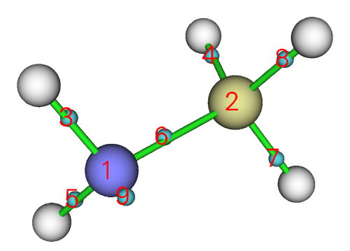
By comparing the graph and content of LMOdip.txt, you can find LMO1 and LMO2, which respectively correspond to core orbitals of N5 and C1, have negligible polarity (i.e. the “norm” are basically zero), reflecting that the LMO centers are very close to the nuclear positions. The LMO9 corresponds to lone pair orbital of N5, its “norm” is as high as 1.35 a.u., showing that the LMO center deviates from N5 nucleus significantly. LMOs 3 and 5 correspond to the N-H bonds, LMOs 4, 7 and 8 correspond to the C-H bonds, it is well known that polarity of C-H should be lower than N-H, this point is well reflected by the difference in their “Norm” values. The “Norm” of LMO6, which corresponds to the C-N bond, is 0.3089, well indicating the fact that C-N is a polar bond.

In addition, in current system the Y coordinates of N5 and C1 are -1.438 and 1.330 Bohr, respectively. The Y component of the bond dipole moment of LMO6 is 0.253, which is an evident positive value. This observation shows that the negative and positive charge centers are on the N5 and C1 sites, respectively, corresponding to the fact that nitrogen has larger electronegativity than carbon.