4.14 Adaptive natural density partitioning (AdNDP) analysis
Theory basis of AdNDP analysis has been introduced in Section 3.17.1, please read it first. Below I will show how to use AdNDP approach to study multi-centers orbitals of a frew practical molecules. More detailed discussions about AdNDP analysis can be found in my blog article "Study multi-center bonds by AdNDP approach as well as ELF/LOL and multi-center bond order" (in Chinese, http://sobereva.com/138).
Note
NOTICE: Using diffuse functions in AdNDP analysis is strongly deprecated, because they often cause numerical problems (which sometimes leads to crash when Multiwfn loading input file) while never improving AdNDP results!
4.14.1 Analyze Li5+ cluster
In Chem. Eur. J., 6, 2982 (2000), the authors showed that Li5+ cluster has two 4-centers 2-electrons (4c-2e) bonds by examining ELF isosurfaces. In present example, we will use AdNDP approach to study this cluster to verify their statement. We first optimize Li5+ cluster under B3LYP/6-311G* level and then compile an input file of single point task for Gaussian. pop=nboread keyword must be specified in route section, and $NBO AONAO DMNAO $END must be added to the end of the input file. Run this file by Gaussian, and then convert check point file to .fch format. The input file, output file and .fch file have been given in "examples\AdNDP" folder.
Boot up Multiwfn and input examples\AdNDP\Li5+.out, and then choose main function 14. After Multiwfn loaded some necessary information, a menu appears. Since this cluster is small, we can directly use exhaustive manner to search all possible 1c-2e, 2c-2e, 3c-2e, 4c-2e and 5c-2e orbitals in turn. We first choose option 2 to search 1c-2e orbitals (namely lone pairs), however, because occupation numbers of all tried 1c orbitals are lower than default threshold (which is a value close to 2.0 and can be adjusted by option 4), the candidate orbitals list shown in front of the menu is still empty. We then choose option 2 twice to search 2c-2e and 3c-2e orbitals in turn, we still cannot find any orbital with high occupation numbers. Next we select option 2 again to search 4c-2e orbitals, this time the candidate orbital list is no longer empty, there are two orbitals in it:
Due to their high occupation number, it clear that they are ideal 4c-2e orbitals, therefore we decide to choose option 0 and input 2 to pick them out from candidate list and save as AdNDP orbitals. After that the list of AdNDP orbitals can be printed by option 5.
You may have noticed that the number of residual valence electrons (shown at the top of the menu) has been updated to 0.020, which is already very close to zero, it is suggested it is meaningless to continue to search 5c-2e orbitals because they would be impossible to be found.
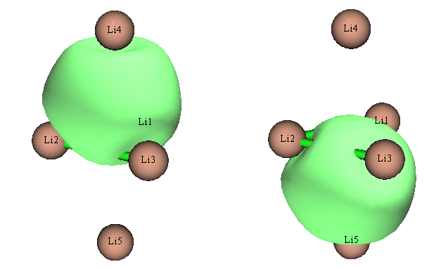
Now you can choose option 7 to visualize the two 4c-2e AdNDP orbitals. In order to calculate orbital wavefunction, Multiwfn needs to load basis set information from corresponding .fch file first. Since Li5+.fch is in the same folder and has identical name as Li5+.out, the .fch file will be directly loaded. When loading is finished, a GUI pops up, which is completely identical to the one of main function 0. AdNDP orbitals can be plotted by selecting corresponding numbers in the right-bottom list. The 0.05 isosurfaces of the two orbitals are shown below.
Grid data of AdNDP orbitals can be exported as Gaussian cube files by option 9, so that you can plot them by some third-part visualization programs such as VMD and Molekel. You need to input orbital index range, assume that we want to output the two 4c-2e AdNDP orbitals we just found, we should input 1,2 and choose a proper grid setting, then they will be exported as AdNDPorb0001.cub and AdNDPorb0002.cub in current folder.
By option 3, you can set the number of centers of multi-centers orbitals in the next exhaustive search. So, assume that you have already known that there are two 4c-2e orbitals in present system, you can directly choose option 3, input 4 and then select option 2 to start the exhaustive search of 4c-2e orbitals, the exhaustive searches of 1c-2e, 2c-2e and 3c-2e orbitals will be skipped.
Evaluating AdNDP orbital energies
It is also possible to obtain energies of the AdNDP orbitals that have been picked out. To realize this, you need to provide additional plain text file containing Fock matrix of present system in lower-triangular sequence, so that orbital energies can be yielded after some transformations of this matrix. The Fock matrix can also be loaded from .47 file. The most straightforward procedure is: Copy examples\AdNDP\Li5+.gjf as examples\AdNDP\Li5+_47.gjf, change last line of it to $NBO archive file=C:\Li5+ $END. Then after running this file by Gaussian, C:\Li5+.47 will be yielded, which is input file of GENNBO program and contains the Fock matrix that we need. Then we choose option "16 Output energy of picked AdNDP orbital" in the AdNDP analysis interface, input the path of the Li5+.47 (which has already been provided in "examples\AdNDP\" folder), Multiwfn will load it and immediately print AdNDP orbital energies, as shown below:
Energy of picked AdNDP orbitals:
Orbital:     1  Energy (a.u./eV):   -0.325776     -8.8648
Orbital:     2  Energy (a.u./eV):   -0.325776     -8.8648
As expected, the two orbitals are degenerated in energy, since they have exactly equivalent shape.
Note
Of course, if you write $NBO DMNAO AONAO archive file=C:\Li5+ $END in the last line of .gjf file, then after running it, not only the output file can be used as input file for AdNDP analysis, but also the .47 file used to derive AdNDP orbital energies will be yielded at the same time.
4.14.2 Analyze B11− cluster
This time, we will try to reproduce the AdNDP analysis result of B11− cluster that given in AdNDP original paper (Phys. Chem. Chem. Phys., 10, 5207 (2008)).
The files needed by this instance, namely B11-.out and B11-.fch can be found in "examples\AdNDP" folder. The geometry was optimized under B3LYP/6-311+G*, while the wavefunction was generated under HF/STO-3G level. You may wonder whether the result is meaningful under such low level of basis set; actually, AdNDP analysis is rather insensitive to basis set quality, even STO-3G is able to produce at least qualitative reasonable result. In addition, using larger basis set will bring additional cost at AdNDP analysis stage.
Boot up Multiwfn and input examples\AdNDP\B11-.out, then choose 14 to enter AdNDP module. As usual, we select 2 to search 1c-2e orbitals first, but we find nothing (this is common case). Then select 2 again to exhaustively search 2c-2e orbitals from the 11 atoms, Multiwfn will totally try 11!/(11-2)!/2!=55 combinations, finally there are nine 2c orbitals present in candidate list (sorted according to occupation number from large to small):
#   9 Occ:  1.9727  Atom:   6B   10B
#   8 Occ:  1.9727  Atom:   5B   11B
#   7 Occ:  1.9742  Atom:   7B    9B
#   6 Occ:  1.9742  Atom:   7B    8B
#   5 Occ:  1.9869  Atom:   2B    6B
#   4 Occ:  1.9869  Atom:   3B    5B
#   3 Occ:  1.9871  Atom:   9B   11B
#   2 Occ:  1.9871  Atom:   8B   10B
#   1 Occ:  1.9942  Atom:   2B    3B
All of them have an occupation number close to 2.0, ostensibly one can directly pick all of them out as AdNDP orbitals, however, it is not recommended to do so, because neighboring orbitals may share partial density. For example, the 1st and the 4th candidate orbitals share partial density, since both of them are related to atom 3. In order to avoid overcount of electrons, firstly you should pick out the first three orbitals by choosing option 0 and input 3, then the density of the first three orbitals will be depleted from density matrix, after that wavefunction and occupation number of remained candidate orbitals will be updated automatically. After that the candidate list becomes
#   6 Occ:  1.9538  Atom:   6B   10B
#   5 Occ:  1.9538  Atom:   5B   11B
#   4 Occ:  1.9556  Atom:   7B    8B
#   3 Occ:  1.9556  Atom:   7B    9B
#   2 Occ:  1.9750  Atom:   2B    6B
#   1 Occ:  1.9750  Atom:   3B    5B
Since some densities have been depleted, occupation number of remaining six candidate orbitals slightly decreased. Now, we pick out the first four candidate orbitals by choosing option 0 and input 4. Although both of 3th and 4th orbitals are related to atom 7, here we have to ignore the slight overcount of electrons, otherwise their degeneration will be broken and thus the final AdNDP pattern will not be consistent with molecular symmetry anymore (you can choose option 8 to carefully inspect candidate orbitals before you decide to pick them out). Finally, we pick out the last two orbitals (i.e. 6B-10B and 5B-11B). Currently the number of residual valence electrons is 16.307, which reveals that it is probable to find several higher number-centers orbitals with nearly two electrons occupied.
Now we select option 2 to start the search of 3c-2e orbitals, the current candidate orbital list is:
#   9 Occ:  1.7399  Atom:   1B    6B   10B
#   8 Occ:  1.7399  Atom:   4B    5B   11B
#   7 Occ:  1.7502  Atom:   1B    3B    4B
#   6 Occ:  1.7502  Atom:   1B    2B    4B
#   5 Occ:  1.8504  Atom:   1B    2B    6B
#   4 Occ:  1.8504  Atom:   3B    4B    5B
#   3 Occ:  1.8603  Atom:   1B    4B    7B
#   2 Occ:  1.8673  Atom:   4B    9B   11B
#   1 Occ:  1.8673  Atom:   1B    8B   10B
After we pick out two orbitals (1B-8B-10B and 4B-9B-11B), one orbital (1B-4B-7B) and two orbitals (3B-4B-5B and 1B-2B-6B) in turn, the highest occupation number of remained candidate orbitals is 1.41, which is obviously too low to be recognized as 3c-2e orbital, so they will not be concerned. Currently the number of residual valence electrons is 7.03.
Then you can start to search higher number of centers orbitals, beware that this is never a trivial task, and there is no absolute rule on how to reasonably pick out candidate orbitals, different picking manners result in different AdNDP patterns. You may have to try many times before finally obtaining an optimal AdNDP pattern. It is recommended to use option 11 to save present density matrix and AdNDP orbital list into memory, so that you need not to worry about improper pick of candidate orbitals, since saved state can be recovered anytime by choosing option 12.
Now choose option 2 to start the search of 4c-2e orbitals, the highest occupation is merely 1.71, none of them could be picked out.
Select option 2 again to search 5c-2e orbitals, you will find many 5c candidate orbitals, the first two have occupation numbers of 1.89, we pick out both of them.
Then choose option 2 to search 6c-2e orbitals, no good candidate can be found, the highest occupation number is only 1.84. Then choose option 2 to search 7c-2e orbitals, we pick the highest occupied one (1.90). Now the residual valence electron is only 1.34, which is much less than 2.0, indicating that no additional 2e AdNDP orbital could be found, therefore now we can end the AdNDP searching procedure. The amount of residual electron reflects the electrons that cannot be fully represented by present AdNDP pattern (analogous to non-Lewis electron in the NBO framework)
By choosing option 5, information of all AdNDP orbitals can be printed out:
#    1 Occ:  1.9942 Atom:   2B    3B
#    2 Occ:  1.9871 Atom:   8B   10B
#    3 Occ:  1.9871 Atom:   9B   11B
#    4 Occ:  1.9750 Atom:   2B    6B
#    5 Occ:  1.9750 Atom:   3B    5B
#    6 Occ:  1.9556 Atom:   7B    9B
#    7 Occ:  1.9556 Atom:   7B    8B
#    8 Occ:  1.9337 Atom:   6B   10B
#    9 Occ:  1.9337 Atom:   5B   11B
#   10 Occ:  1.8673 Atom:   4B    9B   11B
#   11 Occ:  1.8673 Atom:   1B    8B   10B
#   12 Occ:  1.8533 Atom:   1B    4B    7B
#   13 Occ:  1.8451 Atom:   3B    4B    5B
#   14 Occ:  1.8451 Atom:   1B    2B    6B
#   15 Occ:  1.8908 Atom:   1B    2B    6B    8B   10B
#   16 Occ:  1.8908 Atom:   3B    4B    5B    9B   11B
#   17 Occ:  1.9036 Atom:   2B    3B    5B    6B    7B    8B    9B
Total occupation number in above orbitals:   32.6607
Plotting a batch of AdNDP orbitals simultaneously by VMD script
Now you can use option 7 to visualize all picked AdNDP orbitals. However, this time I show how to plot AdNDP orbitals via VMD, which could simultaneously plot a batch of orbitals and the graphical quality is good. VMD can be freely obtained at http://www.ks.uiuc.edu/Research/vmd/.
Choose option 9, select "Medium-quality grid" and then input 1-17 to export all the 17 AdNDP orbitals as cube files in current folder, the format of the file name is AdNDPorb[index].cub. Assume that you have moved all of them to C: directory, you should edit examples\AdNDP\plotAdNDP.vmd and change this line
to
You also need to make sure that in the script, the values after "set istart" and "set iend" have been set to 1 and 17, respectively, so that the cube files from AdNDPorb0001.cub to AdNDPorb0017.cub will be loaded. The positive and negative phases of the orbital isosurfaces are determined by the values after "set posclr" and "set negclr 0", the orbital isovalue is determined by "set isoval"
Now boot up VMD, copy all content in the plotAdNDP.vmd to VMD console window, all cube files of AdNDP orbitals will be loaded into VMD. Now the VMD Main window looks like below
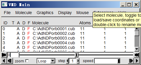
Each entry corresponds to an AdNDP orbital. Currently all the 17 orbitals are shown. If you double click a "D" label, then corresponding orbital will be hidden in the graphical window. In order to show the molecule structure, drag the examples\AdNDP\B11-.xyz into the VMD main window to load it, then enter "Graphics" - "Representation" and change the drawing style as CPK.
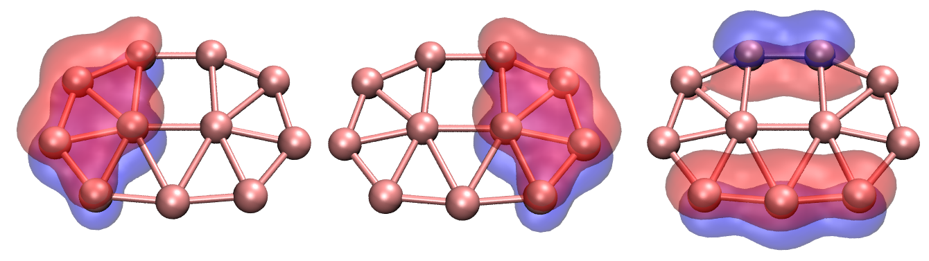
If you make VMD only display all the nine 2c-2e and all the five 3c-2e orbitals, you will see left and right parts of the graph below, respectively
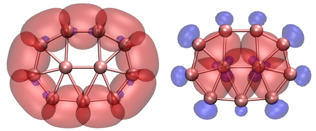
The two 5c-2e and one 7c-2e orbitals are shown below (In the graph the 7c-2e orbital looks like 5c orbital, the main reason is that the isovalue in the plotting script is relatively high, i.e. 0.06).
4.14.3 Analyze phenanthrene
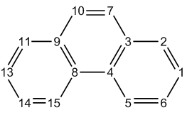
AdNDP analysis of phenanthrene (C14H10, see above) has been given in J. Org. Chem., 73, 9251 (2008), in this section we will repeat their result, you will learn how to use user-directed search. Files used in this example can be found in examples\AdNDP folder with "phenanthrene" prefix.
First we load examples\AdNDP\phenanthrene.out and enter main function 14. In consistency with the previous examples, we select option 2 twice to search 1c orbitals and then search 2c orbitals. No 1c-2e orbitals can be found, while there are 31 candidate 2c orbitals present in the list. Ten of them correspond to C-H σ-bonds and have no overlapping with each other, so we can pick them out first, namely choosing option 0, input 8-15, then choose option 0 again and input 9,10. Next, we successively pick out sixteen 2c candidate orbitals that corresponding to C-C σ-bonds. The most careful way of picking out orbitals is inputting 0 2 0 1 0 2 0 1 0 2 0 2 0 2 0 2 0 2, where space denotes pressing ENTER button once.
Now there are only five orbitals remain:
 #   5 Occ: 1.7182 Atom:   5C    6C
 #   4 Occ: 1.7182 Atom:  14C   15C
 #   3 Occ: 1.7192 Atom:  11C   13C
 #   2 Occ: 1.7192 Atom:   1C    2C
 #   1 Occ: 1.8033 Atom:   7C   10C
The first orbital with occupation number of 1.80 corresponds to the π-bond between C7 and C10, we pick it out now. The occupation numbers of the four remaining orbitals are about 1.72, thus they are not quite ideal 2c-2e bonds, we do not concern them at the moment.
Although we can use option 2 to exhaustively search 3c, 4c, 5c ... orbitals as usual, this may not be a good idea for present system, since user-directed search is often more effective. We first choose option 13 to check population of residual electrons on each atom, see below, this information is usually helpful for guiding users to properly set up exhaustive search list. (Note: The exhaustive search triggered by option 2 is only applied to the atoms in exhaustive search list, which contains all atoms in present system by default)
 1C :  1.0250       2C :  1.0370       3C :  1.0280       4C :  1.0414
 5C :  1.0339       6C :  1.0262       7C :  0.1322       8C :  1.0414
 9C :  1.0280      10C :  0.1322      11C :  1.0370      12H :  0.0117
13C :  1.0250      14C :  1.0262      15C :  1.0339      16H :  0.0121
17H :  0.0113      18H :  0.0117      19H :  0.0126      20H :  0.0111
21H :  0.0121      22H :  0.0113      23H :  0.0111      24H :  0.0126
From above data it is clear that hydrogens have almost vanished population, hence they can be ignored during search. Due to the same reason C7 and C10 can be ignored too. The other atoms, whose occupation numbers are about 1.03, are the carbons composing the two 6-member rings in both sides of the molecule. It can be expected that the two rings may be analogous to benzene ring and hence representing local aromaticity in phenanthrene.
Based on this consideration, we select option 1 and input 1-6 to search AdNDP orbitals for the fragment consisting of atoms 1, 2, 3, 4, 5, 6, we find
...ignored
 #   5 Occ: 0.2157 Atom:   1C    2C    3C    4C    5C    6C
 #   4 Occ: 0.2998 Atom:   1C    2C    3C    4C    5C    6C
 #   3 Occ: 1.8214 Atom:   1C    2C    3C    4C    5C    6C
 #   2 Occ: 1.9850 Atom:   1C    2C    3C    4C    5C    6C
 #   1 Occ: 2.0000 Atom:   1C    2C    3C    4C    5C    6C
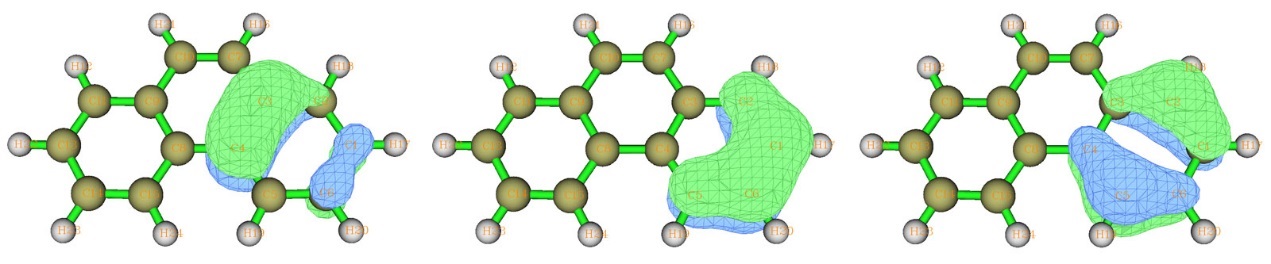
Evidently the first three orbitals are appropriate to be picked out as 6c-2e AdNDP orbitals, so we pick them out now. Their 0.03 isosurfaces are shown below, which look very like π molecular orbitals of benzene, implying that the boundary 6c ring has strong aromaticity as benzene.
Next, via the same way we search 6c-2e orbitals over another boundary ring, namely choose option 1 again and input 8,9,11,13-15, after that we pick out three highest occupied orbitals.
Now the number of residual valence electrons is only 1.15, which is already very small, clearly the AdNDP search should end here. Finally, totally 33 orbitals (27*2c-2e, 6*6c-2e) are found.
Note
When searching 6c-2e orbitals over the ring consisting of atoms 1~6, in fact there is another way to do this (though more cumbersome), namely choose option -1 to enter the interface for defining exhaustive search list, input clean to clean up the default content, then input a 1-6 to add ring atoms 1, 2, 3, 4, 5, 6 into the list, then input x to save and exit. After that, select option 3 and input 6 to set the number of atoms in the next exhaustive search as six, then choose option 2 to search 6-centers orbitals over the ring.
Evaluating AdNDP orbital energies
With similar procedures, we evaluate AdNDP orbital energies like Section 4.14.1. The NBO .47 file containing Fock matrix of current molecule has been provided as examples\AdNDP\phenanthrene.47, which was yielded by examples\AdNDP\phenanthrene_47.gjf. We choose option 16 and input the path of this file, Multiwfn immediately loads Fock matrix from it and outputs the orbital energies:
...(ignored)
 Orbital:    25  Energy (a.u./eV):   -0.685803    -18.6616
 Orbital:    26  Energy (a.u./eV):   -0.685803    -18.6616
 Orbital:    27  Energy (a.u./eV):   -0.260794     -7.0966
 Orbital:    28  Energy (a.u./eV):   -0.348201     -9.4750
 Orbital:    29  Energy (a.u./eV):   -0.255535     -6.9535
 Orbital:    30  Energy (a.u./eV):   -0.264372     -7.1939
 Orbital:    31  Energy (a.u./eV):   -0.348201     -9.4750
 Orbital:    32  Energy (a.u./eV):   -0.255535     -6.9535
 Orbital:    33  Energy (a.u./eV):   -0.264372     -7.1939
As you can see, the orbitals 28-33, which correspond to π orbitals, have energy much higher than σ orbitals. The three π orbitals (28-30) in the left six-membered ring are symmetric to the counterpart orbitals (31-33) in the right six-membered ring. In each side, the two highest lying orbitals (e.g. 32 and 33) are nearly degenerate and evidently higher than the lowest lying one (e.g. 31), this situation is very similar to occupied π orbitals of isolated benzene.
Evaluating composition of AdNDP orbitals
Sometimes composition of AdNDP orbitals is interesting. In the AdNDP module we can directly choose option 15 to analyze orbital composition by NAO method, which has been introduced in Section 3.10.4. NAO method is particularly suitable for analyzing AdNDP orbitals.
Choose option 15, then input index of a picked AdNDP orbital, for example 31, you will see (by default only terms whose absolute contribution > 0.5 % are shown)
    NAO#   Center   Label      Type    Composition
      67    8(C )    px       Val( 2p)     2.247%
      76    9(C )    px       Val( 2p)     1.929%
      94   11(C )    px       Val( 2p)    13.276%
     105   13(C )    px       Val( 2p)    32.846%
     114   14(C )    px       Val( 2p)    34.484%
     123   15(C )    px       Val( 2p)    15.204%

 Condensed NAO terms to shells:
   Atom:     8(C )  Shell:    39( 2p Val)     2.247%
   Atom:     9(C )  Shell:    44( 2p Val)     1.929%
   Atom:    11(C )  Shell:    54( 2p Val)    13.276%
   Atom:    13(C )  Shell:    61( 2p Val)    32.846%
   Atom:    14(C )  Shell:    66( 2p Val)    34.484%
   Atom:    15(C )  Shell:    71( 2p Val)    15.204%

 Condensed NAO terms to atoms:
   Center   Composition
     8(C )     2.251%
     9(C )     1.932%
    11(C )    13.276%
    13(C )    32.849%
    14(C )    34.487%
    15(C )    15.204%
As expected, this π type of 6c-2e orbital purely composes of \(p_{\mathrm{x}}\) natural atomic orbitals, whose axis is perpendicular to the plane of the phenanthrene. This orbital is delocalized over the ring, but mostly distributed on atoms 13 and 14.
Note that there is another way of evaluating AdNDP orbital composition, namely exporting AdNDP orbitals as AdNDP.mwfn in current folder by option 14, and then use this file as input file of Multiwfn and perform orbital composition as usual (via e.g. Mulliken analysis, Hirshfeld analysis and so on, see Section 4.8 for example). For present example, this .mwfn file contains 146 orbitals because there are originally 146 natural atomic orbitals, however only the first 33 orbitals correspond to AdNDP orbitals and thus meaningful.
4.14.4 Analyze Au20 cluster
In this section we perform AdNDP analysis for Au20 cluster, the needed files can be downloaded from http://sobereva.com/multiwfn/extrafiles/Au20.rar.
Boot up Multiwfn and input:
Au20.out // Generated at B3PW91/Lanl2DZ level based on optimized geometry
14 // AdNDP analysis
2 // Search 1-center AdNDP orbitals. 100 candidates are found, whose occupation numbers are very close to 2.0 and thus can be picked out
0 // Pick out orbitals
100 // Pick out all 100 candidate orbitals
2 // Perform exhaustive search of 2-centers orbitals. Nothing can be found
2 // Perform exhaustive search of 3-centers orbitals. Again nothing can be found
2 // Perform exhaustive search of 4-centers orbitals. Now you can see four candidates with 1.84 e and six candidates with 1.7589 e
0 // Pick out orbitals
4 // Pick out first four orbitals. The remaining orbitals now have occupancy of 1.6913, which, although is not quite high, it is still worth to be picked out in current circumstance
0 // Pick out orbitals
6 // Pick out remaining six orbitals.
Plotting AdNDP orbitals
Next we plot all the ten picked 4c-orbitals by VMD using plotting script. We first export their cube files, input below commands
9 // Export cube file of picked AdNDP orbitals
2 // Medium-quality grid, which is adequate for producing smooth orbital isosurface for present system
101-110 // The index range of the picked 4c-orbitals
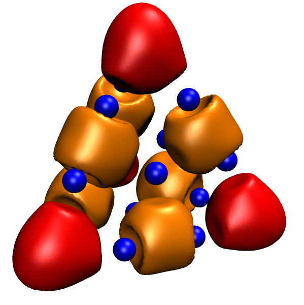
After a while, we have ten cube files in current folder, the first one is AdNDPorb0101.cub, the last one is AdNDPorb0110.cub. We intend to plot the orbitals 101-104 (occ=1.84) using red color while 105-110 (occ=1.69) using orange color so that they can be clearly distinguished.
We edit examples\AdNDP\plotAdNDP.vmd, set "istart" and "iend" to 101 and 104, respectively. Then modify the path after "set name" to make it correspond to the actual path containing the cube files. In addition, add # symbol in the front of the two "mol modmaterial..." lines to comment them out so that the isosurface will be drawn as opaque. After that we boot up VMD, copy all content from the VMD script to the VMD console window, then you will find the first four 4c-orbitals have been shown as isosurfaces in the VMD graphical window.
We also need to plot the orbitals 105-110 on the graph. We set "istart" and "iend" in the script to 105 and 110, respectively. Set "posclr" to 3 to make isosurface color of positive phase to be orange (note that these 4c-orbitals only have positive phase). Set "idinit" to 4, because the systems showing orbital 101, 102, 103 and 104 have already been assigned to be ID=0, ID=1, ID=2 and ID=3 in VMD, respectively, therefore the ID corresponding to the next orbital to be loaded must be 4. Then copy the content of the script to VMD console window to run them, you will find the remaining six 4c-orbitals have also been shown.
Finally, choose "Graphics" - "Representations", click "Create Rep", change "Drawing method" to "CPK". Now you should see the graph below, each red and orange isosurface represents 4c-2e orbital at each vertex and edge of the cluster, respectively.