3.11 Bond order analysis (9)¶

In the bond order analysis module, you can directly select an option to analyze bond order by corresponding method.

If you want to obtain total bond order between atoms in two molecular fragments, you can use option -1 to define fragments 1 and 2 prior to bond order analysis. Then if you choose an option to calculate bond order, the total bond order $I_{\mathrm{RS}}$ between the two fragments will be calculated as follows by summing up interatomic bond orders, and meantime be outputted along with two-center bond orders

\[I_{RS}=\sum_{A\in R}\sum_{B\in S} I_{AB}\]

Note

Evidently, interfragment bond order calculation is not available for multi-center bond order analysis, orbital occupancy-perturbed Mayer bond order and Wiberg bond order decomposition analysis.

3.11.1 Mayer bond order analysis (1)¶

The Mayer bond order between atom A and B is defined as (Chem. Phys. Lett, 97, 270 (1983))

\[I_{AB}=I_{AB}^{\alpha}+I_{AB}^{\beta}=2\sum_{a\in A}\sum_{b\in B}[(\mathbf{P}^{\alpha}\mathbf{S})_{ba}(\mathbf{P}^{\alpha}\mathbf{S})_{ab}+(\mathbf{P}^{\beta}\mathbf{S})_{ba}(\mathbf{P}^{\beta}\mathbf{S})_{ab}]\]

where $P^{α}$ and $P^{β}$ are alpha and beta density matrix respectively, S is overlap matrix. Above formula can be equivalently rewritten using total density matrix P=$P^{α}$+$P^{β}$ and spin density matrix $P^{s}$=$P^{α}$−$P^{β}$

\[I_{AB}=\sum_{a\in A}\sum_{b\in B}[(\mathbf{PS})_{ba}(\mathbf{PS})_{ab}+(\mathbf{P}^{\mathrm{s}}\mathbf{S})_{ba}(\mathbf{P}^{\mathrm{s}}\mathbf{S})_{ab}]\]

For restricted closed-shell circumstance, since spin density matrix is zero, the formula can be simplified to

\[I_{AB}=\sum_{a\in A}\sum_{b\in B}(\mathbf{PS})_{ab}(\mathbf{PS})_{ba}\]

Generally, the value of Mayer bond order is in agreement with empirical bond order; for single, double and triple bonds, the values are close to 1.0, 2.0 and 3.0 respectively. For unrestricted or restricted open-shell wavefunction, alpha, beta and total Mayer bond orders will be outputted separately. By default, only the bonds whose bond order exceed 0.05 will be printed on screen, the threshold can be adjusted by “bndordthres” parameter in settings.ini, you can also select to export full bond order matrix.

Moreover, Multiwfn outputs total and free valences, the former is defined as

\[V_A=2\sum_{a\in A}(\mathbf{PS})_{aa}-\sum_{a\in A}\sum_{b\in A}(\mathbf{PS})_{ab}(\mathbf{PS})_{ba}\]

The latter is defined as

\[F_A=V_A-\sum_{B\neq A}I_{AB}=\sum_{a\in A}\sum_{b\in A}(\mathbf{P}^{\mathrm{s}}\mathbf{S})_{ab}(\mathbf{P}^{\mathrm{s}}\mathbf{S})_{ba}\]

For restricted closed-shell wavefunctions free valences are zero since $P^{s}$=0, thus total valence of an atom is simply the sum of the related bond orders

\[V_A=\sum_{B\neq A}I_{AB}\]

Total valence (also known as atomic valence) measures atomic bonding capacity, while free valence characterizes the remaining ability of forming new bonds by sharing electron pairs.

For unrestricted or restricted open-shell system, there is another way to calculate total bond order rather than summing up alpha and beta bond orders, that is summing up alpha and beta density matrices to form total density matrix first and then calculate Mayer bond order by using restricted closed-shell formula, this treatment is sometimes called “generalized Wiberg bond order“, these total bond orders are printed following the title “Mayer bond order from mixed alpha&beta density matrix”.

Similar to Mulliken population, Mayer bond order and the multi-center bond order described below are sensitive to basis set, so do not use the basis sets having diffuse functions, otherwise the bond order result will be unreliable.

Although Mayer bond order was originally defined for single-determinant wavefunctions, for post-HF wavefunctions, Multiwfn calculates Mayer bond orders via exactly the same formulae as shown above based on corresponding post-HF density matrix. The reasonableness of this treatment has been validated in Chem. Phys. Lett., 544, 83 (2012).

Some applications of Mayer bond order can be seen in J. Chem. Soc., Dalton Trans., 2001, 2095.

Information needed

Basis functions

3.11.2 Multi-center bond order analysis (2, -2, -3)¶

In main function 9 there are three options (2, -2, -3) used to calculate multi-center bond order, they are very similar and will be introduced below in turn. Finally, a notable point about the input order of atomic indices is mentioned.

Option 2: Standard multi-center bond order¶

Multi-center bond index was originally proposed in Struct. Chem., 1, 423 (1990), I prefer to call it as multi-center bond order (MCBO) because of its very similar form with Mayer bond order. In some sense MCBO may be viewed as an extension of Mayer bond order to multi-center cases. Three/four/five/six-center bond orders are defined respectively as

\[\begin{gathered}I_{ABC}=\sum_{a\in A}\sum_{b\in B}\sum_{c\in C}(\mathbf{PS})_{ab}(\mathbf{PS})_{bc}(\mathbf{PS})_{ca}\\ I_{ABCD}=\sum_{a\in A}\sum_{b\in B}\sum_{c\in C}\sum_{d\in D}(\mathbf{PS})_{ab}(\mathbf{PS})_{bc}(\mathbf{PS})_{cd}(\mathbf{PS})_{da}\\ I_{ABCDE}=\sum_{a\in A}\sum_{b\in B}\sum_{c\in C}\sum_{d\in D}\sum_{e\in E}(\mathbf{PS})_{ab}(\mathbf{PS})_{bc}(\mathbf{PS})_{cd}(\mathbf{PS})_{de}(\mathbf{PS})_{ea}\\ I_{ABCDEF}=\sum_{a\in A}\sum_{b\in B}\sum_{c\in C}\sum_{d\in D}\sum_{e\in E}\sum_{f\in F}(\mathbf{PS})_{ab}(\mathbf{PS})_{bc}(\mathbf{PS})_{cd}(\mathbf{PS})_{de}(\mathbf{PS})_{ef}(\mathbf{PS})_{fa}\end{gathered}\]

Similarly, infinite-center bond order can be written as

\[I_{ABCDEF\cdots K}=\sum_{a\in A}\sum_{b\in B}\sum_{c\in C}\cdots\sum_{k\in K}(\mathbf{PS})_{ab}(\mathbf{PS})_{bc}(\mathbf{PS})_{cd}\cdots(\mathbf{PS})_{ka}\]

For open-shell cases, there are two definitions of the MCBO, the first one is the sum of alpha part and beta parts:

\[\begin{aligned}&I_{ABCDEF\cdots K}=I_{ABCDEF\cdots K}^{\alpha}+I_{ABCDEF\cdots K}^{\beta}\\& =2^{n-1}\left[\sum_{a\in A}\sum_{b\in B}\sum_{c\in C}\cdots\sum_{k\in K}(\mathbf{P}^{\alpha}\mathbf{S})_{ab}(\mathbf{P}^{\alpha}\mathbf{S})_{bc}(\mathbf{P}^{\alpha}\mathbf{S})_{cd}\cdots(\mathbf{P}^{\alpha}\mathbf{S})_{ka}\right]\\& +2^{n-1}\left[\sum_{a\in A}\sum_{b\in B}\sum_{c\in C}\cdots\sum_{k\in K}(\mathbf{P}^{\beta}\mathbf{S})_{ab}(\mathbf{P}^{\beta}\mathbf{S})_{bc}(\mathbf{P}^{\beta}\mathbf{S})_{cd}\cdots(\mathbf{P}^{\beta}\mathbf{S})_{ka}\right]\end{aligned}\]

Another definition is using the mixed density matrix, this is not rigorous as above:

\[\begin{gathered}I_{ABCDEF\cdots K}=\sum_{a\in A}\sum_{b\in B}\sum_{c\in C}\cdots\sum_{k\in K}(\mathbf{P}^{\mathrm{mixed}}\mathbf{S})_{ab}(\mathbf{P}^{\mathrm{mixed}}\mathbf{S})_{bc}(\mathbf{P}^{\mathrm{mixed}}\mathbf{S})_{cd}\cdots(\mathbf{P}^{\mathrm{mixed}}\mathbf{S})_{ka}\\ \mathbf{P}^{\mathrm{mixed}}=\mathbf{P}^{\alpha}+\mathbf{P}^{\beta}\end{gathered}\]

For unrestricted or restricted open-shell wavefunction, the output of MCBO analysis consists of four terms, which have been explained above: (1) The result from alpha density matrix (2) The result from beta density matrix (3) The sum of the result of alpha and beta parts (4) The result from mixed alpha&beta density matrix. Commonly, if you are only interested in total MCBO, you should use (3).

Notice that the MCBO for different number of centers are not directly comparable, since the result is not in the same magnitude. However, in Phys. Chem. Chem. Phys., 18, 11839 (2016), it was shown that the normalized MCBO is comparable for different ring size and can be simply calculated as MCB$O^{1/}$ⁿ, where n is the number of centers. For example, at B3LYP/6-31G* level, the MCBO for $H_{3}^{+}$, benzene (6 centers) and naphthalene (10 centers) are 0.2963, 0.0863 and 0.0080, respectively, while the normalized results are 0.667, 0.665 and 0.617, respectively. When MCBO is negative, the normalized value will be calculated as -|MCBO|^1/ⁿ. Commonly, if you need to compare MCBO between different number of centers, you should take the normalized MCBO from the information printed by Multiwfn, else using raw MCBO value is suggested.

Multiwfn is able to automatically search multi-center bonds. If you input -3 when Multiwfn asks you to input atom combination, all three-center bond orders will be calculated, only those larger than the threshold you inputted will be printed. Similarly, four-, five- and six-center bonds can be searched by inputting -4, -5 and -6 respectively. Due to efficiency consideration, the search may not be exhaustive. Also note that the search is based on mixed alpha&beta density matrix for open-shell cases.

There is a hidden option -3 in main function 9, it is used to calculate MCBO under Löwdin orthogonalized basis. The only difference between this option and the option 2 described above is that this option performs Löwdin orthogonalization for basis functions before calculating the MCBO. Since this method does not have obvious advantage over the standard MCBO definition, this option is rarely used and thus invisible in the interface. However, if you have interest, you can have a try.

Option -2: Multi-center bond order in natural atomic orbital (NAO) basis¶

The most severe drawback of the MCBO is its high basis set dependency. In particular, if diffuse functions are presented, then MCBO result may be misleading or completely meaningless. In order to tackle this problem, I proposed an alternative way (to be published) to calculate the MCBO, and the idea is implemented as option -2.

Option -2 is very similar to option 2 (as introduced above), the only difference is that the MCBO is calculated based on natural atomic orbital (NAO) basis rather than based on the basis functions originally defined by the basis set. Since NAO is an orthonormal set and thus overlap matrix S is an identity matrix, the formula can be simplified as (using closed-shell form for example)

\[I_{ABCDEF\cdots K}=\sum_{a\in A}\sum_{b\in B}\sum_{c\in C}\cdots\sum_{k\in K} P_{ab}P_{bc}P_{cd}\cdots P_{ka}\]

The MCBO calculated in this manner has very good stability with respect to change in basis set. Even if diffuse functions are presented the result is still fully reliable. According to my experience, if no basis function shows diffuse character, the results given by option 2 and -2 will be very similar, though not exactly identical.

In order to use option -2, the output file of NBO module embedded in Gaussian or standalone NBO program (namely GENNBO) should be used as input file, and DMNAO keyword must be used to make NBO print density matrix in NAO basis. If you are a Gaussian user, for example, you can use output file of below instance as input file of Multiwfn (DO NOT use .fch file for this analysis!).

#p PBE1PBE/6-311G** pop=nboread

opted

0 1
 C                  0.00000000    1.38886900    0.00000000
... [ignored]
 H                 -2.14060700    1.23588000    0.00000000

$NBO DMNAO $END

In this function, if you only input indices of two atoms, then the result is just Wiberg bond order under NAO basis, which is completely identical to that printed by bndidx keyword of NBO program.

Influence of input order of atomic indices on the result¶

Both the direction (e.g. A,B,C,D vs. D,C,B,A) and permutation (e.g. A,B,C,D vs. B,D,C,A ...) of the inputted atomic indices can influence the calculated MCBO, below I describe this point in detail.

Input direction

Due to the mathematical form of the original MCBO (i.e. the one calculated by option 2), the result of MCBO may rely on input direction. For example, the result yielded by inputting A,B,C,D can be different from that by inputting D,C,B,A. The reason is clear: The term corresponding to A,B,C,D is (PS)_ab(PS)_bc(PS)_cd(PS)_da, while if we invert the input order, the term will become (PS)_dc(PS)_cb(PS)_ba(PS)_ad. Although both P and S are symmetry matrices, their product PS is not necessarily symmetry, so the two terms are not equivalent. In my own viewpoint, in order to obtain more reasonable result, if in a ring the atom connectivity is A-B-C-D-E-F (A also connects to F), one should calculate A,B,C,D,E,F and F,E,D,C,B,A respectively and then take their average. If you want Multiwfn to directly print the averaged value, you can set "iMCBOtype" in settings.ini to 1, in this case you do not need to manually perform the calculation twice, however, of course, the computational cost is doubled compared to normal case.

An advantage of using option -2 to calculate MCBO in NAO basis and using option -3 to calculate it in Löwdin orthogonalized basis is that the result is irrelevant to the input direction, this is because in these cases the overlap matrix S is not explicitly involved and the density matrix P is a symmetry matrix.
Index permutation

Permutation of inputted atomic indices in the calculation of MCBO can significantly alter the result. For example, the result of inputting 1,2,3,4,5,6 may be very different to that of inputting 2,4,3,5,6,1, regardless of which form of MCBO is used. If your aim is to study aromaticity and characterize cyclic delocalization of electrons over a ring, you should input the atomic indices in clockwise or anti-clockwise order, or take their average as mentioned above.

Some people advocated that it is needed to take all possible permutations into account to get a definitive result, see J. Phys. Org. Chem., 18, 706 (2005); that means for a region consisting of six atoms, the bond order of (B,C,A,D,E,F), (C,A,B,D,E,F), (D,B,C,A,F,E) and so on (6!=720 in total) are all required to be taken into account. This definition became known as multi-center index (MCI) in Phys. Chem. Chem. Phys., 18, 11839 (2016). An explicit definition is given below, see Eq. 9 of Phys. Chem. Chem. Phys., 18, 11839 (2016):

\[\mathrm{MCI}=\frac{1}{2n}\sum_{\hat{P}(A,B,C\cdots)} I_{A,B,C\cdots}\]

where n is the number of atoms involved in the calculation, $\hat{P}$ is permutation operator that generates all possible permutation sequences. The MCI is significantly more expensive than the MCBO, and it is not suitable for measuring aromaticity or cyclic delocalization. However, it may be useful in measuring "global" electron delocalization among atoms in a cluster-like region.

If you want to make Multiwfn directly print MCI, you can set "iMCBOtype" in settings.ini to 2, then if you calculate MCBO as usual (via any of options 2, -2 and -3), the printed result will correspond to MCI.

Finally, it is worth to note that MCBO may be marginally negative in some cases. If you did not employ diffuse functions, or the MCBO was calculated based on NAOs, then you can simply view the very small negative MCBO as zero. For three-center cases, if MCBO is an evident negative value, then it is implied that there is a three-center four-electron (3c-4e) interaction (e.g. CO₂).

Information needed

Basis functions (options 2, -3), NBO output file with DMNAO keyword (option -2)

Appendix: The extremely efficient implementation of MCBO in Multiwfn¶

According to the expression, the computational cost of MCBO seems to increase exponentially with the increase of the number of atoms in the ring, making its evaluation infeasible for large rings. Thanks to the special implementation of MCBO proposed by me, the cost of MCBO in Multiwfn grows only linearly with number of ring members, computational time is negligible even for a ring consisting of many dozens of atoms! The algorithm is described as follows.

Five-center MCBO is taken as an example here, whose original definition is

\[I_{ABCDE}=\sum_{a\in A}\sum_{b\in B}\sum_{c\in C}\sum_{d\in D}\sum_{e\in E}(PS)_{ab}(PS)_{bc}(PS)_{cd}(PS)_{de}(PS)_{ea}\]

which can be reformulated as

\[I_{ABCDE}=\sum_{a\in A}\sum_{b\in B}(PS)_{ab}\sum_{c\in C}(PS)_{bc}\sum_{d\in D}(PS)_{cd}\sum_{e\in E}(PS)_{de}(PS)_{ea}\]

If an intermediate matrix A is fully calculated and stored in memory, whose element is expressed as

$A_{d,a}=\sum_{e\in E}(PS)_{de}(PS)_{ea}$,

then MCBO can be simplified to

\[I_{ABCDE}=\sum_{a\in A}\sum_{b\in B}(PS)_{ab}\sum_{c\in C}(PS)_{bc}\sum_{d\in D}(PS)_{cd}A_{d,a}\]

Next, if an intermediate matrix B is fully calculated and stored in memory, whose element is expressed as

$B_{c,a}=\sum_{d\in D}(PS)_{cd}A_{d,a}$,

then MCBO can be simplified to

\[I_{ABCDE}=\sum_{a\in A}\sum_{b\in B}(PS)_{ab}\sum_{c\in C}(PS)_{bc}B_{c,a}\]

Furthermore, if an intermediate matrix C is fully calculated and stored in memory, whose element is expressed as

$C_{b,a}=\sum_{c\in C}(PS)_{bc}B_{c,a}$,

then MCBO can be finally simplified to

\[I_{ABCDE}=\sum_{a\in A}\sum_{b\in B}(PS)_{ab}C_{b,a}\]

It is clear that using the intermediate matrices A, B, C, MCBO can be evaluated in a quite simple manner, while construction of A, B, C is also very cheap. The formal cost of this reformulation of MCBO only increases linearly with number of atoms, and thus can be easily applied for a ring even consisting of more than 100 atoms.

In order to prove the correctness and the significant value of the special implementation of MCBO in Multiwfn, a comparison of the results and time consumption for calculating MCB$O^{1/}$ⁿ of cyclo[n]carbon system at ωB97XD/def2-TZVP level is given below. In the table, “old” denotes the direct programming based on the original equation of MCBO, which was conducted using Multiwfn 3.6 (in which the current algorithm has not been available), “current” denotes the algorithm described above. Intel i9-13980HX CPU was used for the test. It can be seen that the two algorithms give exactly the same result, however the cost of the “old” algorithms is already high for cyclo[8]carbon (even using a small basis set like 6-31G*, MCBO usually can at most be used for a ring containing a dozen atoms). In contrast, the current algorithm can exactly calculate MCBO of cyclo[48]carbon only within 1 second!

n	Wall time (s)		MCB$O^{1/}$ⁿ
n	old	current	old	current
6	<1s	<1s	0.639945	0.639945
8	358s	<1s	0.578652	0.578652
10		<1s		0.649397
12		<1s		0.611403
14		<1s		0.637272
24		<1s		0.561782
48		<1s		0.549418

3.11.3 Wiberg bond order analysis in Löwdin orthogonalized basis (3)¶

Wiberg bond order is defined as follows, see footnote in Tetrahedron, 24, 1083 (1968)

\[I_{AB}=\sum_{a\in A}\sum_{b\in B} P_{ab}^2\]

The original definition of Wiberg bond order is only suitable for the wavefunction represented by orthogonal basis functions such as most semiempirical wavefunctions, and only defined for restricted closed-shell system. Actually, Mayer bond order can be seen as a generalization of Wiberg bond order, for restricted closed-shell system and orthonormal basis function (namely S matrix is identity matrix) cases their results are completely identical.

In this function, Multiwfn first orthogonalizes basis functions by Löwdin method and then performs usual Mayer bond order analysis. The threshold for printing is controlled by “bndordthres” in settings.ini too.

As shown in J. Mol. Struct. (THEOCHEM), 870, 1 (2008), the Wiberg bond order calculated in this manner, say $W_{L}$, has much less sensitivity to basis set than Mayer bond order (whereas for small basis sets, their results are close to each other). One should be aware that $W_{L}$ tends to overestimate bond order for polar bonds in comparison with Mayer bond order.

Commonly, if there is no special reason, using Mayer bond order is preferred.

Notice that numerous papers used NBO program to calculate Wiberg bond order, the result must be somewhat different to that produced by present function, because in NBO program the Wiberg bond orders are calculated under the basis of natural atomic orbitals (NAO), which are generated by OWSO orthogonalization method. Multiwfn is also possible to calculate Wiberg bond order in NAO basis, and furthermore, the result can be decomposed as atomic orbital pair contributions, see Section 3.11.8 for details.

Information needed

Basis functions

3.11.4 Mulliken bond order analysis (4) and decomposition (5)¶

Mulliken bond order is the oldest bond order definition, it is defined as

\[I_{AB}=\sum_i\eta_i\sum_{a\in A}\sum_{b\in B}2C_{a,i}C_{b,i}S_{a,b}=2\sum_{a\in A}\sum_{b\in B} P_{a,b}S_{a,b}\]

Mulliken bond order has low agreement with empirical bond order, it is deprecated for quantifying bonding strength, for which Mayer bond order always performs better. However, Mulliken bond order is a good qualitative indicator for bonding (positive value) and antibonding (negative value). The threshold for printing results is controlled by “bndordthres” parameter in settings.ini.

Mulliken bond order is easy to be decomposed to orbital contributions, the contribution from orbital i to bond order AB is

\[I_{AB}^i=\eta_i\sum_{a\in A}\sum_{b\in B}2C_{a,i}C_{b,i}S_{a,b}\]

From the decomposition, we can know which orbitals are favourite and unfavourable for specific bonding.

Information needed

Basis functions

3.11.5 Orbital occupancy-perturbed Mayer bond order (6)¶

Orbital occupancy-perturbed Mayer bond order was first proposed in J. Chem. Theory Comput., 8, 908 (2012). Put simply, by using this method one can obtain how large is the contribution from specific orbital to Mayer bond order.

Orbital occupancy-perturbed Mayer bond order can be written as

\[I_{A,B}^*=I_{AB}^{*,\alpha}+I_{AB}^{*,\beta}=2\sum_{a\in A}\sum_{b\in B}[(\mathbf{P}_X^{\alpha}\mathbf{S})_{ba}(\mathbf{P}_X^{\alpha}\mathbf{S})_{ab}+(\mathbf{P}_X^{\beta}\mathbf{S})_{ba}(\mathbf{P}_X^{\beta}\mathbf{S})_{ab}]\]

The only difference between this definition and Mayer bond order shown in Section 3.11.1 is that $P^{α}$ and $P^{β}$ have been replaced by ${\mathbf{P}}_{X}^{\alpha}$ and ${\mathbf{P}}_{X}^{\beta}$ respectively. $P_{X}$ stands for the density matrix generated when occupation number of a specific orbital is set to zero. The difference between ${I}_{A,B}^{*}$ and Mayer bond order can be regarded as a measure of contribution from the orbital to Mayer bond order. Bear in mind, because Mayer bond order is not a linear function of density matrix, the sum of ${I}_{A,B}^{*}$ for all orbitals is not equal to Mayer bond order generally.

In Multiwfn, you only need to input indices of two atoms, then ${I}_{A,B}^{*}$ for all occupied orbitals and the difference between ${I}_{A,B}^{*}$ and Mayer bond order will be outputted. The more negative (positive) the difference, the more beneficial (harmful) to the bonding due to the existence of the orbital.

You can also use another way to calculate ${I}_{A,B}^{*}$, that is using wavefunction modification module (main function 6) to manually set occupation number of a specific orbital to zero, and then calculate Mayer bond order as usual, but this manner may be tedious if you want to calculate ${I}_{A,B}^{*}$ for many orbitals.

This kind of analysis is illustrated in Section 4.9.1 and Section 4.19.3.

Information needed

Basis functions

3.11.6 Fuzzy bond order (7)¶

Fuzzy bond order (FBO) was first proposed by Mayer in Chem. Phys. Lett., 383, 368 (2004):

\[\begin{gathered}B_{AB}=B_{AB}^{\alpha}+B_{AB}^{\beta}=2\sum_{\mu}\sum_{\nu}[(\mathbf{P}^{\alpha}\mathbf{S}^A)_{\mu\nu}(\mathbf{P}^{\alpha}\mathbf{S}^B)_{\nu\mu}+(\mathbf{P}^{\beta}\mathbf{S}^A)_{\mu\nu}(\mathbf{P}^{\beta}\mathbf{S}^B)_{\nu\mu}]\\ S_{\mu\nu}^A=\int w_A(\mathbf{r})\chi_\mu^*(\mathbf{r})\chi_\nu(\mathbf{r})\mathrm{d}\mathbf{r}\end{gathered}\]

where S is the overlap matrix between basis functions in fuzzy atomic spaces. In Multiwfn, Becke's fuzzy atomic space with sharpness parameter k=3 in conjunction with modified CSD radii is used for calculating FBO. (See Section 3.18.0 for introduction of fuzzy atomic space).

Commonly the magnitude of FBO is close to Mayer bond order, especially for low-polar bonds, but much more stable with respect to the change in basis set. According to the comparison between FBO and delocalization index (DI) given in J. Phys. Chem. A, 109, 9904 (2005), FBO is essentially the DI calculated in fuzzy atomic space. See Section 3.18.5 for details about DI.

Calculation of FBO requires performing Becke's DFT numerical integration, due to which the computational cost is larger than evaluation of Mayer bond order. By default, 40 radial points and 230 angular points are used for numerical integration. This setting is able to yield accurate enough results in general. If you want to further refine the result, you can set the number of radial and angular points by "radpot" and "sphpot" in settings.ini manually, and ensure that "iautointgrid" has been set to 0.

The threshold for printing results is controlled by “bndordthres” parameter in settings.ini.

Information needed

GTFs, atom coordinates

3.11.7 Laplacian bond order (8)¶

In J. Phys. Chem. A, 117, 3100 (2013) (http://pubs.acs.org/doi/abs/10.1021/jp4010345), I proposed a novel definition of covalent bond order based on the Laplacian of electron density ${\mathrm{\nabla }}^{2}\rho$ in fuzzy overlap space, called Laplacian bond order (LBO). The LBO between atom A and B can be simply written as

\[L_{A,B}=-10\times\int_{\nabla^2\rho<0} w_A(\mathbf{r})w_B(\mathbf{r})\nabla^2\rho(\mathbf{r})\mathrm{d}\mathbf{r}\]

where w is a smoothly varying weighting function proposed by Becke and represents fuzzy atomic space, hence $w_{A}$$w_{B}$ corresponds to fuzzy overlap space between A and B. Note that the integration is only restricted to negative part of ${\mathrm{\nabla }}^{2}\rho$. The physical basis of LBO is that the larger magnitude the integral of negative ${\mathrm{\nabla }}^{2}\rho$ in the fuzzy overlap space, the more intensively the electron density is concentrated in the bonding region, and therefore, the stronger the covalent bonding.

In the original paper of LBO, the reasonableness and usefulness of LBO were demonstrated by applying it to a wide variety of molecules and by comparing it with many existing bond order definitions. It is shown that LBO has a direct correlation with bond polarity, bond dissociation energy and bond vibrational frequency. The computational cost of LBO is low, also LBO is insensitive to the computational level used to generate electron density. In addition, since LBO is inherently independent of wavefunction, one can in principle obtain LBO by making use of accurate electron densities derived from X-ray diffraction data.

In Multiwfn, Becke's fuzzy atomic space with sharpness parameter k=3 in conjunction with modified CSD radii is used for calculating LBO. (See Section 3.18.0 for detail about fuzzy atomic space). The threshold for printing results is controlled by “bndordthres” parameter in settings.ini.

Note that in current implementation, LBO is particularly suitable for organic systems, but not for ionic bonds since in these cases a better definition of atomic space should be used to faithfully exhibit actual atomic space. LBO is also not very appropriate for studying the bond between two very heavy atoms (heavier than Ar), because these bonds are often accompanied by insignificant charge concentration in the fuzzy overlap space, even though the bonding is doubtless covalent.

A good application example of LBO is Carbon, 165, 468 (2020), in which LBO was employed to characterize the bonding between two different kinds of C-C bonds in cyclo[18]carbon.

Information needed

GTFs, atom coordinates

3.11.8 Decompose Wiberg bond order in NAO basis as atomic orbital pair contributions (9)¶

Theory¶

As mentioned in Section 3.11.3, Wiberg bond order is expressed as

\[I_{AB}=\sum_{a\in A}\sum_{b\in B} P_{ab}^2\]

The data is calculated for atomic pairs. Since the expression is simply a linear combination of square of density matrix element, it is straightforward to decompose Wiberg bond order as basis function pair contribution (this idea is to be published). For example, $P_{\mathrm{ab}}$² is simply the contribution from interaction between basis functions a and b. Since one-to-one correspondence between basis function and atomic orbital is lacking when extended basis set is used, in order to make the decomposition method full of physical meaning, the decomposition is best to be carried out under natural atomic orbitals (NAOs). Each non-Rydberg type of NAO uniquely corresponds to an atomic orbital, thus, by above decomposition method, Wiberg bond order at the atomic orbital scale can be obtained.

In addition, contribution from interaction between atomic orbital shells i and j can be obtained as$\sum_{a\in\mathrm{shell}\ i}\sum_{b\in\mathrm{shell}\ j} P_{ab}^2$.

By the way, it is also possible to decompose multi-center bond order as atomic orbital contribution. For example, three-center bond order is expressed as

\[I_{ABC}=\sum_{a\in A}\sum_{b\in B}\sum_{c\in C} P_{ab}P_{bc}P_{ca}\]

Clearly, $P_{\mathrm{ab}}$$P_{\mathrm{bc}}$$P_{\mathrm{ca}}$ can be regarded as the contribution from interaction between NAOs a, b and c. However, decomposition of multi-center bond order under NAO basis has not been implemented.

Usage¶

After entering this function, simply input indices of two atoms, the nonnegligible contribution from NAO pairs and NAO shell pairs together with total Wiberg bond will be printed.

You can also input -1 to input atom indices to define two fragments, then NAO shell contributions between the two fragments to the interfragment Wiberg bond order will be given.

The input file of this function is completely identical to the option -2 described in Section 3.11.2, namely the output file of NBO program containing density matrix information (i.e. "DMNAO" keyword is required).

An illustrative example of this decomposition analysis is given in Section 4.9.4.

3.11.9 Intrinsic bond strength index (IBSI) (10)¶

Theory¶

The intrinsic bond strength index (IBSI) was proposed in J. Phys. Chem. A, 124, 1850 (2020) to quantify strength of chemical bonds, it may also be used to compare strength of weak interactions. The IBSI was originally defined in the framework of independent gradient model (IGM), which is very detailedly described in Section 3.23.5. The IBSI is expressed as

\[\mathrm{IBSI}=\frac{(1/d^2)\int\delta g^{\mathrm{pair}}\mathrm{d}\mathbf{r}}{(1/d_{\mathrm{H}_2}^2)\int\delta g^{\mathrm{H}_2}\mathrm{d}\mathbf{r}}\]

where d is the distance between the two atoms for which the interaction is to be studied. The integral in the numerator is equivalent to the atomic pair δg index defined by me between the two atoms, see Section 3.23.6 for detail. The denominator is the data for reference system, the ${d}_{{\mathrm{H}}_{2}}$ and the integral are the bond length and atomic pair δg index of H₂ in its equilibrium structure, respectively. In the original paper of IBSI, it was shown that the IBSI value is modestly positively correlated with strength of covalent bond. Furthermore, it was found that magnitude of IBSI of transition metal coordinate bond is markedly smaller than that of covalent bond, and magnitude of IBSI of weak interactions is even much lower, this feature of IBSI may be used to distinguish type of interaction.

Implementation¶

It is important to note that in the IBSI paper the authors calculated the IBSI using the IGM based on gradient-based partition (IG$M^{\mathrm{GBP}}$), however this form of IGM is not supported by Multiwfn. Currently Multiwfn supports the original form of IGM, namely IGM based on promolecular approximation (IG$M^{\mathrm{pro}}$), and also supports IGM based on Hirshfeld partition of molecular density (IGMH), as well as mIGM. Different forms of IGM correspond to different ways of evaluating gradient of atomic density, and thus the value of the integral in the IBSI expression is correspondingly different. In Multiwfn, the IBSI can be computed based on IG$M^{\mathrm{pro}}$, IGMH, and mIGM, their results are very different, I found the result based IG$M^{\mathrm{pro}}$ is obviously closer to the original paper of IBSI.

Usage¶

To calculate IBSI, you simply need to enter main function 9 and select subfunction 10, then select option 0 to start calculation.

Before calculation, Multiwfn asks you to choose quality of integration grid, evidently the better the grid, the higher the cost, while the more accurate the result. According to my experience, for IG$M^{\mathrm{pro}}$, "medium quality" is already able to give a quantitatively accurate result; while for IGMH and mIGM, at least "high-quality" should be used if you have requirement on accuracy.

You can choose which form of IGM will be used in the IBSI calculation by option 2. If the input file contains wavefunction information, by default IGMH is used, while if the input file only contains geometry information (e.g. .pdb, .mol, .xyz...), IG$M^{\mathrm{pro}}$ or mIGM can be used. Note that IGMH is much more expensive than IG$M^{\mathrm{pro}}$, since its formula to evaluate gradient of atomic density is much more complicated.

If you are only interested in the interactions in a local region, you can choose option 3 to define the region to be studied, only the IBSI between the atoms in the defined fragment will be evaluated and outputted, the cost is correspondingly lower than the IBSI calculation for the whole system, especially when the system is huge.

The reference value can be set by option 4, it corresponds to the denominator of the IBSI formula. Of course, this value must be different for IG$M^{\mathrm{pro}}$, IGMH, and mIGM. The default reference values were calculated for H₂ with experimental bond length (0.74144 Å), in the IGMH case B3LYP/6-311G** wavefunction was employed. Commonly, the reference value does not need to be changed. However, for calculating IBSI in terms of IGMH, if you want to obtain the reference value at your current calculation level to pursue stricter result, you can load wavefunction file of H₂, then enter the present function, set reference value to 1.0, then use option 0 to start to calculate IBSI, the result can be employed as reference value for studying practical molecules.

In order to avoid excessive output, by default only the data for the atomic pairs with separation smaller than 3.5 Å are printed, because IBSI should be negligible if the separation is larger. If you need to adjust the distance printing threshold, use option 5.

Example of calculating IBSI is given in Section 4.9.6.

Information needed

Atom coordinates (for IBSI based on IG$M^{\mathrm{pro}}$ and mIGM), GTF information (for IBSI based on IGMH)

3.11.10 AV1245 index (approximate multi-center bond order for large rings) and AVmin¶

Theory¶

The multi-center bond order (MCBO), as introduced in Section 3.11.2, is a very rigorous and popular way of characterizing aromaticity. In Phys. Chem. Chem. Phys., 18, 11839 (2016), the authors proposed the AV1245 index to quantify aromaticity for large rings, it can be regarded as an approximation of MCBO.

Note

The original key advantage of AV1245 over MCBO is that the computational cost of AV1245 only increases linearly with number of atoms, while the cost of MCBO is usually prohibitively high for a ring composed of more than 11~12 atoms. However, since Multiwfn 3.8, the computational time of MCBO also becomes linearly proportional to ring members and thus MCBO can be easily employed for very large rings, the value of AV1245 becomes much less obvious.

The definition of AV1245 in the original paper is "average all the 4c-ESI values along the ring that keeps a positional relationship of 1, 2, 4, 5". Here I clarify its definition. As an instance, for below ring,

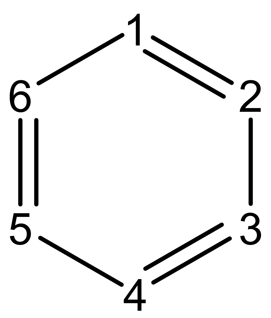
Benzene ring with the atom numbering used for the AV1245 index

its AV1245 is calculated as

AV1245=[ESI(1,2,4,5)+ESI(2,3,5,6)+ESI(3,4,6,1)+ESI(4,5,1,2)+ESI(5,6,2,3)+ESI(6,1,3,4)] / 6

where the nc-ESI (n-center electron sharing index) can be directly obtained via the multi-center bond order with all possible permutations (namely I ^perm, see Section 3.11.2 for detail) by below relationship

\[\mathrm{ESI}=\frac{2}{(n-1)!}I^{\mathrm{perm}}\]

where n is the number of atoms. Evidently, 4c-ESI = (4c-$I^{\mathrm{perm}}$) / 3.

The central idea of AV1245 is based on the fact that in an aromatic ring, the resonance between 1-2 bond and 4-5 bond is strong, as illustrated below. This feature can be captured by ESI(1,2,4,5).

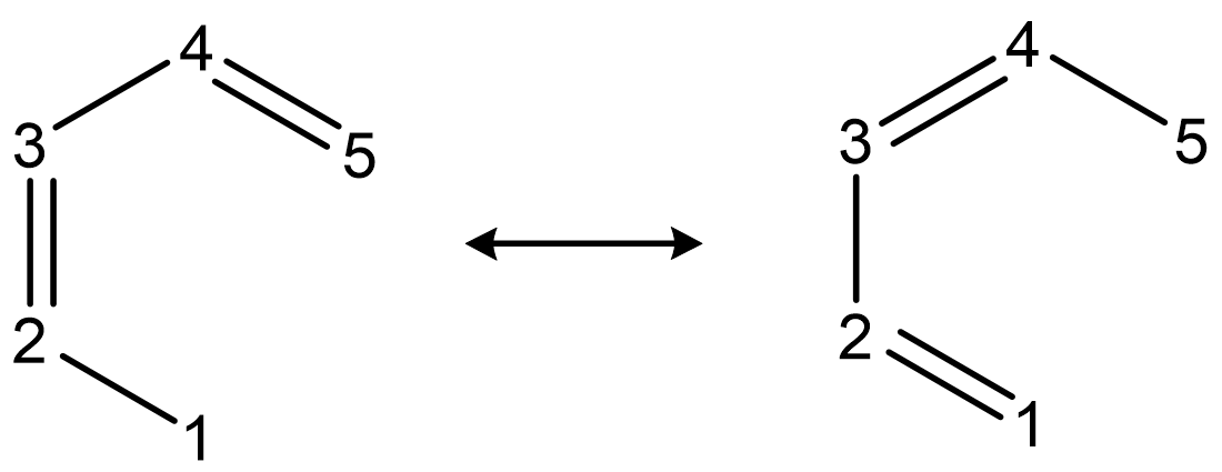
Resonance between the 1-2 and 4-5 bonds of a five-membered ring

Larger value of AV1245 of a cyclic path implies stronger delocalization and thus larger aromaticity of the ring. Since magnitude of AV1245 is small, it is often multiplied by 1000 when presenting the data.

It is worth to note that in the original paper of AV1245, the MCBO was calculated in terms of atomic overlap matrix under AIM partition, this way of calculation is not only expensive but complicated. In Multiwfn, the MCBO involved in the AV1245 is calculated in usual way, namely based on density matrix and overlap matrix. Since in this case the calculation of 4-center I ^perm is fairly cheap, the AV1245 can be quickly obtained even for large systems and macro-rings. However, due to the difference in the calculation of MCBO, the result of AV1245 produced by Multiwfn is smaller than that in the original paper. In addition, when directly calculating AV1245 by Multiwfn (in other words, calculating AV1245 in original basis functions), the employed basis set should not contain diffuse functions, otherwise the AV1245 will be meaningless.

Multiwfn also supports calculating AV1245 in natural atomic orbital (NAO) basis, in this case reasonable result can be obtained even if diffuse functions are presented. If there is no diffuse function, the result calculated in original basis functions and that in NAO basis is nearly the same.

The AVmin index was proposed in J. Phys. Chem. C, 121, 27118 (2017) and further discussed in Phys. Chem. Chem. Phys., 20, 2787 (2018). It corresponds to minimal absolute value of all 4c-ESIs involved in the calculation of AV1245. Unlike AV1245, AVmin quantifies lowest degree of conjugation in the whole pathway, therefore it has unique value in distinguishing aromaticities of different delocalization pathways, since according to common intuition, aromaticity of a path should be predominated by the local region mostly disconnecting the delocalization over the whole path. In other words, AVmin is able to determine the bottleneck of aromaticity of a given path.

Usage¶

Calculating AV1245 and AVmin in original basis functions

You should enter subfunction 19 of main function 200, then input indices of the atoms in the ring in the order of connectivity (clockwise or counterclockwise along the ring). After that, the AV1245 together with its constituent 4c-ESI values as well as AVmin will be outputted

Note

Multiwfn provides convenience for inputting the atomic indices for large rings. If you input d first and press ENTER button, then you can input the atomic indices in arbitrary order, because in this case the actual order will be automatically guessed according to interatomic connectivity. However, this input mode cannot be used when any atom in the ring connects to more than two other atoms in the ring.
Calculating AV1245 and AVmin in NAO basis

The operation process is the same as "Calculating AV1245 and AVmin in original basis functions", however, you should use output file of standalone NBO program or the NBO module embedded in quantum chemistry codes as input file of Multiwfn, and meantime the "DMNAO" keyword must be employed in the NBO analysis. Note that in this case the aforementioned "d" mode of index inputting is not available.

Examples of employing AV1245 and AVmin to study aromaticity of small rings and large rings are given in Section 4.9.11.

Information needed

Atom coordinates, basis functions

3.11.12 Delocalization index (DI) between AIM basins¶

The concept of delocalization index (DI) is given in Section 3.18.5. The DI calculated between atoms-in-molecules (AIM) basins, namely the basins partitioned for electron density, is a quantification of number of electron pairs shared by different atoms, and can also be regarded as a metric of bond order. However, this kind of DI tends to be lower for bonds with higher bond polarity. Due to this reason, for nonpolar bonds, DI is usually very close to Mayer bond order and fuzzy bond order, while for polar bonds, the discrepancy can be quite large.

The basin analysis module can calculate DI, as described in Section 3.20. However, the most straightforward way of obtaining DI between atoms is directly using the dedicated function, namely subfunction 12 of main function 9. You will be asked to select grid quality, the better the quality, the higher the cost, while more accurate the result. Uniform with atomic centered integration grids are employed to calculate DI in this function.

Information needed

Atom coordinates, basis functions