3.9 Population analysis and calculation of atomic charges (7)

This module is used to calculate population number of basis functions, shells, atoms, fragments, or atomic charges. There are some points that should be noted:

Regardless of which subfunction you choose, if you want to evaluate fragment charge/population (the sum of charge/population of the atoms in a fragment), you should select option "-1 Define fragment" first and input atom indices to define the fragment. Then once the calculation of atomic charges is finished, fragment charge will be printed along with atomic charges. If your input file is .chg or .pqr, which contains atomic charge information, this option also automatically prints the sum of atomic charges of the atoms in the fragment.

After atomic charge calculation, you can choose to output atomic coordinates with calculated charges to [name of loaded file].chg file in current directory, see Section 2.5 for detail about .chg format.

If the file loaded when Multiwfn boots up is .chg format, you can use option "-2 Calculate interaction energy between fragments based on atomic charges" in present function to evaluate interfragment electrostatic interaction energy between two given fragments by classic Coulomb formula (see below) using the atomic charges in this .chg file.

\[E_{\mathrm{Coul-int}}=\sum_{A\in\mathrm{frag1}}\sum_{B\in\mathrm{frag2}}\frac{q_A q_B}{\left|\mathbf{R}_A-\mathbf{R}_B\right|}\]

This feature is useful for studying electrostatic interaction components in total molecular interaction energy, as well as evaluating intermolecular exciton coupling energy based on atomic transition charges (see Section 4.A.9 on how to derive them).

If you are not familiar with atomic charges, it is strongly suggested to read my review article, which very comprehensively introduced concepts, characteristics, applications, calculation methods of atomic charges:

Tian Lu,* Qinxue Chen, Partial Charges, In Exploring Chemical Concepts Through Theory and Computation. WILEY-VCH GmbH: Weinheim (2024); pp. 161-187. DOI: 10.1002/9783527843435.ch6.

3.9.1 Hirshfeld atomic charge (1)

Hirshfeld is a very popular atomic population method based on deformation density partition, Hirshfeld charge is defined as (Theor. Chim. Acta (Berl.), 44, 129 (1977))

\[q_A=-\int w_A^{\mathrm{Hirsh}}(\mathbf{r})\rho_{\mathrm{def}}(\mathbf{r})\mathrm{d}\mathbf{r}\]

where

\[\begin{gathered}\rho^{\mathrm{def}}(\mathbf{r})=\rho(\mathbf{r})-\rho^{\mathrm{pro}}(\mathbf{r})\\ \rho^{\mathrm{pro}}(\mathbf{r})=\sum_A \rho_A^{\mathrm{free}}(\mathbf{r}-\mathbf{R}_A)\end{gathered}\]

It can also be rewritten as follows to make its physical meaning clearer

\[\begin{aligned}&q_A=-\int w_A^{\mathrm{Hirsh}}(\mathbf{r})[\rho(\mathbf{r})-\rho^{\mathrm{pro}}(\mathbf{r})]\mathrm{d}\mathbf{r}\\ &=-\int w_A^{\mathrm{Hirsh}}(\mathbf{r})\rho(\mathbf{r})-\rho_A^{\mathrm{free}}(\mathbf{r}-\mathbf{R}_A)\mathrm{d}\mathbf{r}\\ &=-\int w_A^{\mathrm{Hirsh}}(\mathbf{r})\rho(\mathbf{r})\mathrm{d}\mathbf{r}+\int\rho_A^{\mathrm{free}}(\mathbf{r}-\mathbf{R}_A)\mathrm{d}\mathbf{r}\\ &=-p_A+Z_A\end{aligned}\]

where \(p_{A}\) is population number of the atom in actual chemical system. Z is nuclear charge, which equals the number of electrons carried by the atom in its free state.

The advantages of Hirshfeld population are:

1. Result is qualitatively consistent with general chemical concepts such as electronegativity rule.

2. The weighting function w for space partition has clear physical meaning.

3. Unlike the methods based on integrating electron density such as AIM charge, what the Hirshfeld charge reflects is the amount of transferred electron density during molecule formation, the density not transferred is not involved.

4. Insensitive to the quality of wavefunction.

5. Although calculating Hirshfeld charge needs integration in real space, due to the smooth integrand, sophisticated density functional theory (DFT) grid-based integration schemes can be directly used, so Hirshfeld population is high-efficient.

6. The wide application field. Deformation density data can also be obtained by X-ray crystallography experiments. Moreover, the applicability of Hirshfeld population is not constrained by the type of wavefunction, the method can be directly applied to solid system, where the wavefunction generally be described by plane-wave functions.

The disadvantages of Hirshfeld population are the charge is always too small and the poor reproducibility of observable quantities, such as molecular dipole moment and ESP, the reason is Hirshfeld population completely ignores atomic dipole moments.

After calculation, if the printed sum of all Hirshfeld charges is very close to integer, that means the quadrature is accurate; if not, that means the outputted Hirshfeld charges are unreliable, you need to increase the density of integration points by setting “radpot” and “sphpot” to larger value and calculate again. For balancing computational time and accuracy, the default value of “radpot” and “sphpot” are 75 and 434, respectively, you can set them to 100 and 590 respectively to obtain more accurate results.

An example is given in Section 4.7.1.

Information needed

GTFs, atom coordinates

3.9.2 Voronoi deformation density (VDD) atom population (2)

The only difference between VDD and Hirshfeld population is the weighting function w. In VDD population, the Voronoi cell-like partition is used, each cell corresponds to an atom, see J. Comput. Chem., 25, 189 (2004) for details.

The results of VDD population are similar to Hirshfeld population in common, because the magnitude of deformation density is always small, so there is no significant change in charges when different weighting functions are used. The outputted terms are identical to Hirshfeld population. Personally, I suggest you use Hirshfeld population instead of VDD.

Note that if the sum of VDD atomic charge deviates from molecular net charge evidently, that means the numerical integration accuracy is not satisfactory, and hence you should enlarge "sphpot" parameter in settings.ini to improve the result. "radpot" parameter also influences the result, but not so significantly as "sphpot".

Information needed

GTFs, atom coordinates

3.9.3 Mulliken atom & basis function population analysis (5)

Theory

Mulliken analysis is the oldest population method based on orbital wavefunction, supported by almost all quantum chemistry packages.

Orthonormality condition of spin orbital wavefunction entails \(1=\int\left|\varphi(\mathbf{r})\right|^2\mathrm{d}\mathbf{r}\), if we assume that the orbital is real type and insert the linear combination equation \(\varphi_i(\mathbf{r})=\sum_a C_{a,i}\chi_a(\mathbf{r})\) into it, we get

\[1=\int\left(\sum_a C_{a,i}\chi_a(\mathbf{r})\right)^2\mathrm{d}\mathbf{r}=\sum_a C_{a,i}^2+\sum_a\sum_{b\neq a}C_{a,i}C_{b,i}S_{a,b}=\sum_a C_{a,i}^2+2\sum_a\sum_{b>a}C_{a,i}C_{b,i}S_{a,b}\]

where \(S_{a,b}=\int\chi_a(\mathbf{r})\chi_b(\mathbf{r})\mathrm{d}\mathbf{r}\), the normality of basis functions is used in derivation. The first term is “local term”, denotes the net population of each basis function in orbital i, the second term is “cross term”, denotes the shared electrons between basis function pairs in orbital i. Certainly the local terms should be completely attributed to corresponding basis functions, however for cross terms the partition method is not unique. Mulliken defined the population of basis function a in spin orbital i as

\[\Theta_{i,a}=C_{a,i}^2+\sum_{b\neq a}C_{a,i}C_{b,i}S_{a,b}\]

That is each cross term \(2C_{a,i}C_{b,i}S_{a,b}\) is equally partitioned to corresponding two basis functions.

The population number of atom A is simply the sum of population numbers of all basis functions attributed to atom A in all orbitals. Mulliken atomic charge is defined as

\[q_A=Z_A-\sum_i n_{i,A}=Z_A-\sum_i\eta_i\sum_{a\in A}\Theta_{i,a}\]

where η is orbital occupation number, \(n_{i,A}\) is the contribution from orbital i.

Mulliken analysis is not ideal for practical application due to these shortcomings:

1. Poor reproducibility of observable properties such as molecular dipole moment

2. The “equal partition” of cross term has no strict physical meaning

3. Very high basis set dependence. In particular, diffuse functions must not be presented, otherwise the result will be misleading.

4. Occasionally, meaningless results occur (population numbers are negative).

Usage

Since amount of outputted information is huge for large systems, before selecting below subfunctions, you can use option -1 to change the default output destination from screen to a specific plain text file.

• Subfunction 1 (Output Mulliken population and atomic charges): Population of basis functions, population of basis function shells, population of each angular moment of atomic orbitals, as well as atomic charges are printed.

• Subfunction 2 (Output gross atomic population matrix and decompose it): Gross atom population matrix is printed, from which you can get local terms of each atom (diagonal element) and cross terms between each atomic pair (non-diagonal element multiplies 2). The matrix element is defined as

  \[\Omega_{A,B}=\sum_i\Omega_{A,B}^i=\sum_i\eta_i\sum_{a\in A}\sum_{b\in B}C_{a,i}C_{b,i}S_{a,b}\]

  Note that the last row of outputted matrix is the sum of corresponding column elements, that is the total population number of corresponding atom. You can also choose to decompose the matrix to contribution of each occupied orbital, the Ω matrices will be outputted to groatmdcp.txt in current directory.

  By the way, the quantity \(2{\Omega}_{A,B}^{i}\) is just the Mulliken bond order between atom A and B contributed from orbital i, as we will see in Section 3.11.4.

• Subfunction 3 (Output gross basis function population matrix and decompose it): Gross basis function population matrix can be outputted by this option for further analyzing detail of electron distribution, the matrix element is defined as

  \[\Gamma_{a,b}=\sum_i\Gamma_{a,b}^i=\sum_i\eta_i C_{a,i}C_{b,i}S_{a,b}\]

  Likewise, in subfunction 3, the last row of the outputted matrix is total population number of corresponding basis function. You can also choose to output contribution of each occupied orbital, namely \({\Gamma}_{a,b}^{i}\), to grobasdcp.txt in current directory (notice that this file is extremely large even for medium-sized system).

• Subfunction 4 (Output orbital contributions to atomic populations to atmpopdcp.txt): This option is used to output contributions of occupied orbitals to atomic populations, namely all \(\sum_i\eta_i\sum_{a\in A}\Theta_{i,a}\) terms, to atmpopdcp.txt in current folder.

An example of Mulliken population analysis is given in Section 4.7.0.

Information needed

Basis functions

3.9.4 Löwdin atom & basis function population (6)

The only difference between Löwdin and Mulliken population analysis is whether Löwdin orthogonalization is performed first. In Löwdin orthogonalization, the transformation matrix is

\[\mathbf{X}=\mathbf{U}\mathbf{s}^{1/2}\mathbf{U}^{\mathrm{T}}\]

where U is eigenvector matrix of overlap matrix, matrix s is diag(λ₁, λ₂...), where {λ} is eigenvalue set of overlap matrix. After Löwdin orthogonalization, the overlap matrix becomes identity matrix, and new coefficient matrix is \(X^{-1}\)C.

Ostensibly, Löwdin population avoids the partition for cross terms since they have become zero, actually, the partition step is no more than hidden in the orthogonalization. Since Löwdin orthogonalization still has no strong physical meaning, it cannot make conclusion that Löwdin population is better than Mulliken. In view of practical results, one also found Löwdin charges have no evident advantages relative to Mulliken charges, though some people argued that Löwdin charges have better basis set stability and reproducibility of molecular dipole moment. Besides, Mayer et. al. found Löwdin population has rotation dependence to some extent when Cartesian type Gaussian basis functions are used, however the dependency can be safely ignored in generally, for detail please see Chem. Phys. Lett., 393, 209 (1968) and Int. J. Quantum Chem., 106, 2065 (2006).

Information needed

Basis functions

3.9.5 Modified Mulliken atom population defined by Ros & Schuit (SCPA) (7)

Some people had proposed several different partition methods of cross term to improve Mulliken analysis, they are generally called as modified Mulliken population analysis (MMPA). In the method proposed by Ros and Schuit (Theo. Chim. Acta, 4, 1 (1966)), the composition of basis function a in orbital i is defined as

\[\Theta_{i,a}=\frac{C_{a,i}^2}{\sum_b C_{b,i}^2}\]

only the squares of coefficients are presented in the formula, so this method is also called C-squared Population Analysis (SCPA). By inserting the identity

\[1=\sum_a C_{a,i}^2+\sum_a\sum_{b\neq a}C_{a,i}C_{b,i}S_{a,b}\]

into the right most of above formula, Θ can be rewritten as

\[\Theta_{i,a}=C_{a,i}^2+\frac{C_{a,i}^2}{\sum_b C_{b,i}^2}\sum_a\sum_{b\neq a}C_{a,i}C_{b,i}S_{a,b}\]

It is clear that when calculating composition of basis function a in orbital i, what is partitioned is not the cross terms between atom a and other atoms, but the total cross term of all atomic pairs. The SCPA atomic charges can be calculated in the same manner as Mulliken charges by using the newly defined Θ. Relative to Mulliken population, the advantage of SCPA is that negative value of population number never occurs.

Information needed

Basis functions

3.9.6 Modified Mulliken atom population defined by Stout & Politzer (8)

Stout and Politzer defined the Θ as (Theor. Chim. Acta, 12, 379 (1968))

\[\Theta_{i,a}=C_{a,i}^2+\sum_{b\neq a}\frac{C_{a,i}^2}{C_{a,i}^2+C_{b,i}^2}2C_{a,i}C_{b,i}S_{a,b}\]

That is cross terms are partitioned according to the ratio of the squares of corresponding coefficients. Ostensibly, this definition has more consideration on the unbalanced nature of cross term, however in practical applications the results are even worse than Mulliken, therefore this method is rarely used now. Besides, Grabenstetter and Whitehead had pointed out that this MMPA definition has unitary transformation dependence, so if the molecule is rotated the results will change (the dependence is remarkable and cannot be ignored).

Information needed

Basis functions

3.9.7 Modified Mulliken atom population defined by Bickelhaupt (9)

The population number of a basis function defined in Organometallics, 15, 2923 (1996) is

\[\Lambda_a=\sum_i\eta_i C_{a,i}^2+\sum_{b\neq a}w_{a,b}\sum_i 2\eta_i C_{a,i}C_{b,i}S_{a,b}\]

where the weight of basis function a for partitioning the total cross term between a and b in all orbitals is

\[w_{a,b}=\frac{\sum_k\eta_k C_{a,k}^2}{\sum_i\eta_i C_{a,i}^2+\sum_j\eta_j C_{b,j}^2}\]

Essentially, it is equivalent to define Θ as

\[\Theta_{i,a}=C_{a,i}^2+\sum_{b\neq a}w_{a,b}2C_{a,i}C_{b,i}S_{a,b}\]

This method is similar to the MMPA defined by Stout and Politzer, the difference is in the latter the weight \(w_{a,b}\) is only related to local terms of basis functions a and b in current orbital, while in present method the weight is related to total local terms of basis functions a and b.

Information needed

Basis functions

3.9.8 Becke atomic charge with atomic dipole moment correction (10)

In the paper J. Chem. Phys., 88, 2547 (1988), Becke proposed a weighting function for converting whole space integral to multiple single-center spherical integrals, although the weighting function is not intended for population analysis, Multiwfn still makes an attempt to use this weighting function as atomic space to obtain atomic charges. The Becke charge can be defined as

\[q_A=Z_A-\int w_A(\mathbf{r})\rho(\mathbf{r})\mathrm{d}\mathbf{r}\]

The radii used for evaluating the Becke weighting function (or say Becke atomic space) can be controlled by uses, see corresponding options shown on screen. For details about Becke weighting function please see J. Chem. Phys., 88, 2547 (1988) or Section 3.18.0. According to my experiences, by using the default "modified CSD" radii, Becke charge is reasonable for typical organic systems, but not very appropriate for ionic systems. For details about the "modified CSD" radii, see the end of Section 3.18.0.

After the Becke charges are calculated, atomic dipole moment correction will be performed automatically. The correction process is identical to the one used for correcting Hirshfeld charge (see next section). After the correction the charges will have better electrostatic potential reproducibility and can exactly reproduce molecular dipole moment.

Information needed

GTFs, atom coordinates

3.9.9 Atomic dipole moment corrected Hirshfeld atomic charges (ADCH, 11)

Basic characteristics and usage

The main reason why Hirshfeld charges are too small and have poor reproducibility of observable quantity is that atomic dipole moments are completely neglected. In the ADCH method proposed by me (J. Theor. Comput. Chem., 11, 163 (2012)), atomic dipole moment of each atom is expanded to correction charges placed at neighbouring atoms, then ADCH charge is just the sum of original Hirshfeld charge and correction charge. ADCH atomic charges are very reasonable in chemical sense, molecular dipole moment is exactly reproduced, the reproducibility of ESP is close to the atomic charges obtained from fitting ESP. Compared to another method that try to improve Hirshfeld charges, namely Hirshfeld-I (see Section 3.9.13), the computational cost of ADCH charge is negligible. Owing to its many advantages, ADCH is a highly recommended atomic charge model. For an extensive comparison of atomic charge models, see Acta Phys. -Chim. Sin, 28, 1 (2012).

Before doing ADCH correction, Hirshfeld charge will be calculated first. In the summary field, “corrected” and “before” correspond to ADCH charge and Hirshfeld charge respectively. At final stage, the “Error” means the difference between molecular dipole moment produced by ADCH charges and the one produced by actual electron density, “Error” is always equal to or very close to zero, because ADCH charges in principle exactly reproduce molecular dipole moment.

If you would like to obtain the detail of charge transfer between atoms in the atomic dipole moment correction process, you can set “ishowchgtrans” in settings.ini to 1.

Algorithm detail about expanding atomic dipole moment

Full details of ADCH charge can be found from its original paper, here I only mention how the atomic dipole moment correction (ADC) is realized.

Assume that we want to expand atomic dipole moment of atom A as correction charges, clearly, the sum of all correction charges should be zero, and the dipole moment evaluated based on the correction charges should be exactly equal to atomic dipole moment, namely below conditions should be satisfied

\[\begin{gathered}\sum_B\Delta q_{A\to B}=0\\ \unicode{x1D6CD}_A=\sum_B\Delta q_{A\to B}\mathbf{R}_B\end{gathered}\]

where Δ\(q_{A}\)_→B is transferred charge from atom A to B, in other words, it is the correction charge on atom B due to A. The index B cycles all atoms in the system. \(R_{B}\) is relative coordinate (column vector) of atom B with respect to atom A

The correction charges are expected to be distributed only around atoms neighbouring to A, this could be realized by minimizing function F:

\[F=\sum_B\frac{(\Delta q_{A\to B})^2}{\upsilon_{AB}}+\alpha\sum_B\Delta q_{A\to B}+\beta(\unicode{x1D6CD}_A-\sum_B\Delta q_{A\to B}\mathbf{R}_B)\]

where α and β are Lagrangian multipliers used to satisfy the two constraint conditions, the υ_AB is a function that decreases rapidly as increase of distance between A and B, and its detailed form is dependent on atomic radii of A and B, see original paper of ADCH for more information. Obviously, this design of F suppresses occurrence of large correction charge on the atoms far away from atom A.

It is shown that after some manipulations, the working equation of evaluating Δ\(q_{A}\)_→B is

\[\Delta q_{A\to B}=\frac{\upsilon_{AB}}{\sum_B\upsilon_{AB}}\left[(\mathbf{R}_B-\left\langle\mathbf{R}_B\right\rangle)^{\mathrm{T}}\cdot\Lambda^{-1}\cdot\unicode{x1D6CD}_A\right]\]

where superscript "T" is sign of transpose, and

\[\begin{gathered}\Lambda=\left\langle\mathbf{R}_B\cdot(\mathbf{R}_B)^{\mathrm{T}}\right\rangle-\left\langle\mathbf{R}_B\right\rangle\left\langle\mathbf{R}_B\right\rangle^{\mathrm{T}}\\ \left\langle\mathbf{R}_B\right\rangle=\frac{\sum_B\upsilon_{AB}\mathbf{R}_B}{\sum_B\upsilon_{AB}},\quad\left\langle\mathbf{R}_B\cdot(\mathbf{R}_B)^{\mathrm{T}}\right\rangle=\frac{\sum_B\upsilon_{AB}\mathbf{R}_B\cdot(\mathbf{R}_B)^{\mathrm{T}}}{\sum_B\upsilon_{AB}}\end{gathered}\]

If atom A is in local planar region, the Λ matrix will be exactly or almost singular matrix, in this case inversed matrix of Λ obviously cannot be obtained. Notice that the solution to this problem in current implementation is slightly different to the one introduced in the ADCH original paper. In current Multiwfn, the Λ matrix is first diagonalized, the eigenvalues with absolute value less than 10^-5 will be simply set to zero (the corresponding eigenvector typically perpendicular to the local plane of atom A), and remaining eigenvalues are inversed, now this matrix has corresponded to the Λ^-1 in the new local coordinate. Then \({\mathbf{R}}_{B}-\left\langle {\mathbf{R}}_{B} \right\rangle\) and µ_A are transformed to the new local coordinate by doing left multiplication of transpose of eigenvector matrix of Λ on them. Finally, the Δ\(q_{A}\)_→B is obtained using above formula.

An example of calculating ADCH charges is given in Section 4.7.2.

Information needed

GTFs, atom coordinates

3.9.10 CHELPG (Charges from electrostatic potentials using a grid-based method) ESP fitting atomic charge (12)

Theory

CHELPG (J. Comput. Chem., 11, 361 (1990)) is one of most widely used electrostatic potential (ESP) fitting charge models. Compared to CHELP and Merz-Kollman methods, CHELPG charges have better rotational invariance, mostly due to the fitting points are distributed in cubic grid manner.

In CHELPG model, a box is defined first to enclose the whole molecule, extension distance in each side is 2.8 Å, see the red box in the following picture

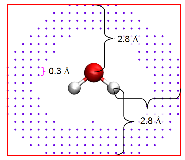
Fitting points are evenly distributed in the box, the default spacing is 0.3 Å. For any fitting point, if the distance between the point and any nucleus is smaller than vdW radius of the atom, or the distances between the point and all nuclei are larger than 2.8 Å, then the fitting point will be discarded. The purple dots shown above are finally used fitting points.

Like other ESP fitting methods, in CHELPG, the deviation function shown below is minimized to make the ESP calculated by atomic charges (\(V_{q}\)) close to the ESP calculated based on wavefunction (V) as good as possible.

\[F(q_1,q_2\cdots q_N)=\sum_i\left[V_q(\mathbf{r}_i)-V(\mathbf{r}_i)\right]^2\]

where \(r_{i}\) is coordinate of fitting point i. {q} are fitted point charges, their positions are referred to as fitting centers. Notice that q does not necessarily correspond to atomic charge, the fitting centers can be defined at arbitrary positions.

It can be shown that the minimization of F could be formulated to the following matrix equation

\[\mathbf{A}\mathbf{q}=\mathbf{B}\]

which can be further explicitly written as

\[\begin{bmatrix}A_{11}&A_{12}&\cdots&A_{1N}&1\\A_{21}&A_{22}&\cdots&A_{2N}&1\\\vdots&\vdots&\ddots&\vdots&1\\A_{N1}&A_{N2}&\cdots&A_{NN}&1\\1&1&1&1&0\end{bmatrix}\begin{bmatrix}q_1\\q_2\\\vdots\\q_N\\\lambda\end{bmatrix}=\begin{bmatrix}B_1\\B_2\\\vdots\\B_N\\q_{\mathrm{tot}}\end{bmatrix}\]

with

\[\mathbf{A}_{A,B}=\sum_i\frac{1}{r_{iA}r_{iB}}\qquad\mathbf{B}_A=\sum_i\frac{V(\mathbf{r}_i)}{r_{iA}}\qquad q_{\mathrm{tot}}=\sum_A q_A\]

where A and B are indices of fitting centers and N is total number of fitting centers. The column vector q is what we need, its first N elements correspond to charges of the fitting centers. The q could be easily evaluated as q=\(A^{-1}\)B.

Usage

In the interface there are many options which are introduced below.

• Option 1: If selecting this option, Multiwfn will start to calculate ESP value at each fitting point, then fitted atomic charges of all fitting centers will be outputted on screen. RMSE and RRMSE are also outputted automatically, they measure quality of fitting, the smaller value suggests that the fitted charges have better ESP reproducibility. RMSE and RRMSE are defined as (where N is the number of fitting points)

  \[\begin{gathered}\mathrm{RMSE}=\sqrt{\frac{\sum_i\left[V_q(\mathbf{r}_i)-V(\mathbf{r}_i)\right]^2}{N}}\\ \mathrm{RRMSE}=\sqrt{\frac{\sum_i\left[V_q(\mathbf{r}_i)-V(\mathbf{r}_i)\right]^2}{\sum_i V(\mathbf{r}_i)^2}}\end{gathered}\]

• Options 2~4: These options are used to set parameters for distributing fitting points. The default values are reasonable and should not be changed without special reasons.

• Option 4: If you hope fitting points only distribute over a certain fragment, you can select this option and input atom indices, then a fitting point will be taken into account only if the atom closest to it belongs to the given atom list.

• Option 5: During the ESP fitting, three kinds of ESP can be calculated and used, namely "Nuclear + Electronic" (default), "Electronic" and "Transition electronic". Commonly you should not change this option. The "Transition electronic" should be chosen if you want to evaluate the so-called TrEsp (transition charge from electrostatic potential), please check Section 4.A.9 for details.

• Option 6: If it is switched to "Yes", then after calculation, coordinates with ESP values of all fitting points can be exported to ESPfitpt.txt or ESPfitpt.pqr in current folder, the former is more readable, while the latter can be directly loaded into VMD program to visualize the fitting points (and can be colored according to the "charge" column, which records ESP values). In addition, fitting points with absolute difference between exact ESP and the ESP evaluated based on atomic charges can be exported to ESPerr.pqr so that ESP reproduction error in various molecular regions can be visualized in VMD. See Section 4.7.8 for illustration.

• Option 8: If it is switched to "Yes", then additional constraints are applied so that the fitted atomic charges will exactly reproduce the electric dipole moment calculated based on wavefunction. The idea comes from J. Comput. Chem., 11, 297 (1990). Note that this type of constraint is usually unimportant, because ESP fitting charges computed in the common manner already have good capability to reproduce dipole moment.

• Option 10: Choose the atomic radii used in fitting. The atomic radii employed in fitting affects the distribution of fitting points, and thus influence the resulting charges. There are three modes that can be chosen to set the radii:

  (1) This is default mode, the radii defined in original paper of CHELPG are used. However, only the elements in the first three rows are defined, if your system contains other elements, Multiwfn will ask you to input their vdW radii in turn. If you do not have proper radii in hand, you can directly press ENTER button, then vdW radius of UFF forcefield of corresponding element multiplied by 1/1.2 will be used, which is commonly a reasonable choice.

  (2) Employing the UFF radii scaled by 1/1.2 for all elements. The UFF radii can be found in Table 1 of UFF original paper J. Am. Chem. Soc., 114, 10024 (1992).

  (3) Load radii of all elements involved in present system from external file. Multiwfn will ask you to input the file path during fitting, the format of the file should like follows, the unit of the radii should be in Å, all elements in the system must be defined:

  H 1.2
  O 1.8
  Cu 2.2
  

• Option -1: For flexibility consideration, by using this option, coordinates of fitting points are allowed to be read from external file to replace the CHELPG fitting points. The format of the file should be

  numdata
  X  Y  Z  [ESPval]                    ← For fitting point 1
  X  Y  Z  [ESPval]                    ← For fitting point 2
  ...
  

  where the ESPval is an optional term, which denotes precalculated ESP value at corresponding point. If numdata is a negative value, then the ESP values used in charge fitting will be read from the fourth column rather than calculated by Multiwfn.

• Option -2: If you have special reasons (e.g. you want to place additional fitting centers at lone pair or σ-hole region to enhance description of ESP around corresponding region), then coordinates of additional fitting centers can be read from external file by using this option. The format of the file should be

  numdata
  X  Y  Z                    ← For additional fitting center 1
  X  Y  Z                    ← For additional fitting center 2
  ...
  

  where numdata denotes how many entries are in this file. X, Y, Z are coordinates (in Å).

• Option -3: If you simply want to examine reproducibility for ESP at the fitting points of given atomic charges, then you can use this option to load atomic charges from specific .chg file. Then when you select option 1 to start the ESP fitting process, no ESP fitting charges will be yielded, only the RMSE and RRMSE of the given atomic charges will be outputted (note that if you have chosen option -2 to load additional fitting centers, then the number of charges in the loaded .chg file should be identical to the total number of fitting centers). If you only want to study reproducibility of ESP for the fitting points around specific fragment, you can choose option 4 and input the atom indices.

An example is given in Section 4.7.1.

Information needed

GTFs, atom coordinates

3.9.11 Merz-Kollmann (MK) ESP fitting atomic charge (13)

Merz-Kollmann (MK) charge is another well-known charge model derived from ESP fitting, see J. Comput. Chem., 11, 431 (1990). The only difference between MK and CHELPG is grid setting. In MK, the fitting points are evenly distributed on the layers of 1.4, 1.6, 1.8 and 2.0 times the vdW radius of each atom, if distance between a fitting point and any atom is smaller than 1.4 times of its vdW radius, then this fitting point will be discarded.

In the MK module of Multiwfn, the density of points per Ų on the MK layers can be set by option 2, the number of layers and the scale factor of atomic vdW radii used to define the layers can be set by option 3, the atoms used to construct the MK fittings points can be set by option 4. For description of other options and outputs, see the last section.

Like the CHELPG module, in the MK module you can also choose the mode for determining atomic radii used in the fitting by option 10. Notice that the original paper of MK method does not explicitly present atomic radii. In Multiwfn, the default MK radii for the first and second rows and P, S, Cl are in line with those in MK code of Gaussian, while the default radii for Na-Si are defined as 1.57, 1.65, 1.65, 1.80 Å, respectively.

In the example in Section 4.7.8, I exemplified how to use the MK module to investigate ESP reproducibility of given atom charges on all MK fitting points and on the fitting points corresponding to specific atoms. In addition, the example showed how to visualize ESP reproduction error at various molecular regions.

Information needed

GTFs, atom coordinates

3.9.12 AIM atomic charge (14)

AIM (Atoms-in-molecules) population corresponds to the number of electrons in AIM basin, and accordingly, subtracting AIM population from nuclear charge yields AIM charge, which is also sometimes incorrectly referred to as Bader charge. AIM charges can be calculated in basin analysis module, please check the example given in 4.17.1 on how to do. Related theories and algorithms of the basin analysis module are introduced in Section 3.20. However, in Multiwfn, the most convenient way of obtaining AIM charges is directly using subfunction 14 of main function 7. In this case, you only need to choose grid quality, then AIM charges will be calculated and printed. Atomic-center + uniform integration grids with exact refinement of basin boundaries are automatically employed.

An example is given in Section 4.7.11.

Information needed

GTFs, atom coordinates

3.9.13 Hirshfeld-I atomic charge (15)

Hirshfeld-I (HI) method was proposed in J. Chem. Phys., 126, 144111 (2007), it is an important extension of Hirshfeld method. It is believed that the atomic space defined by Hirshfeld is not quite ideal, because it does not respond to the actual molecular environment. In HI, atomic spaces are gradually refined via an iterative scheme. After convergence, the final HI atomic spaces are evidently more physically meaningful than the Hirshfeld ones.

There are some variants of HI method, including the Hirshfeld-E proposed in J. Chem. Theory Comput., 9, 2221 (2013), the Hirshfeld-Iλ proposed in J. Comput. Chem., 32, 1561 (2011) and the fractional occupation Hirshfeld-I (FOHI) proposed in J. Chem. Theory Comput., 7, 1328 (2011). Also, there is an iterative atomic space method named iterated stockholder atoms (ISA), which is closely related to HI, see Chem. Commun., 2008, 5909.

Basic theory of HI method

In HI method, the weighting function of atom A at iteration n is defined as

\[w_A^{(n)}(\mathbf{r}-\mathbf{R}_A)=\frac{\rho_A^{(n-1)}(\mathbf{r}-\mathbf{R}_A)}{\sum_B\rho_B^{(n-1)}(\mathbf{r}-\mathbf{R}_B)}\equiv\frac{\rho_A^{(n-1)}(\mathbf{r}-\mathbf{R}_A)}{\rho_{\mathrm{pro}}^{(n-1)}(\mathbf{r})}\]

where r and R denote spatial coordinate and position of atomic nucleus, respectively. The atomic density involved in HI is obtained by linear interpolation between spherically averaged free-state atomic density of adjacent charge states:

\[\rho_A^{(n)}(r)=(q_{\mathrm{up}}-q_A^{(n-1)})\rho_{A,\mathrm{low}}^{\mathrm{free}}(r)+(q_A^{(n-1)}-q_{\mathrm{low}})\rho_{A,\mathrm{up}}^{\mathrm{free}}(r)\]

where \(q_{\mathrm{high}}\) and \(q_{\mathrm{low}}\) are upper and lower integer of atomic charge of atom A at n-1 iteration, while \({\rho}_{A\mathrm{,up}}^{\mathrm{free}}\) and \({\rho}_{A\mathrm{,low}}^{\mathrm{free}}\) are spherically averaged atomic density of atom A at these two charged states, respectively. For example, if atom A carries charge of 0.2 at n-1 step, then its radial atomic density at step n will be computed as

\[\rho_A^{(n)}(r)=0.8\times\rho_{A,q=0}^{\mathrm{free}}(r)+0.2\times\rho_{A,q=+1}^{\mathrm{free}}(r)\]

Before the HI iteration, radial densities of all atoms are initialized to their neutral state.

Based on HI atomic weighting functions, HI atomic charges can be straightforwardly obtained. The HI iteration continues until all atomic charges converged to a given criterion.

Note

It is clear that the HI atomic charges yielded at the first iteration are in principle identical to Hirshfeld charges. However, this is not exactly true in Multiwfn, because currently the rule of generating spherically averaged free-state atomic density involved in HI is not completely identical to that used in Hirshfeld, but the difference is very small and can be ignored. It is never incorrect to directly take the atomic charges printed at the first iteration of HI as Hirshfeld charges.

Usage

After entering the HI analysis module, you will find many options, you can adjust convergence criterion and maximum number of cycles, also you can switch the algorithm for realizing HI iterations (see below), and you can decide if printing atomic charges every iteration.

If you select option 0, Multiwfn will start the HI calculation. Before this, Multiwfn first checks atomic radial density files (.rad) in "atmrad" folder, if they are available for all elements in the current system, HI calculation will directly start; if they are not available, Multiwfn will try to calculate atomic .wfn files by invoking Gaussian and convert them to .rad files, and then start the HI iterations.

After convergence of HI iterations, HI atomic charges and fragment charge/population (if you have defined fragment) are printed. Note that the printed HI atomic charges have been properly normalized to eliminate noise of numerical integration (i.e. making sum of HI population of all atoms equal to total number of electrons). Finally, you can select if outputting resulting atomic charges as .chg file.

Note

There is an option "-3 Switch if speeding up calculation using distance cutoff". By default, this treatment is enabled to significantly reduce costs for large systems. If you find the HI charges are problematic or the calculation cannot be normally finished, you can select this option once to disable this treatment and retry. Alternatively, you can select it twice, then you will be prompted to input a cutoff value for this treatment, the larger the value, the more accurate the result and more robust the calculation will be, however, at the expense of increasing computational cost. The default cutoff is 2.0, which should be very safe for almost all cases.

About preparing atomic radial density files (.rad files)

Before igniting HI iteration, atomic radial density files (.rad files) must be available for all elements in the systems at different charged states. There are three ways to provide them:

• Using built-in .rad files

  The easiest way of providing the .rad files is simply copying the "atmrad" folder from "examples" directory to current folder, then Multiwfn will directly utilize the .rad files in it during HI calculation. This "atmrad" folder contains .rad file of all elements (except for lanthanides and actinides) of all possible charged states, therefore in this case HI charges can be directly computed without any additional step.

  Note

  The .rad files in this folder were carefully generated based on highly accurate densities. Specifically, elements of the first three rows were calculated at PBE0/def2-QZVPP level, all other main group elements were calculated by PBE0/ANO-RCC with DKH2 relativistic Hamiltonian, while all transition metal atoms were calculated by PBE0/Sapporo-DK3-QZP-2012 with DKH2. For each element of each charged state, ground state spin multiplicity was employed, and meantime wavefunction stability test and wavefunction optimization were carried out to make sure that the wavefunction is stable and thus the resulting radial density is realistic.

• Let Multiwfn automatically invoke Gaussian to generate .rad files

  If needed .rad files are not found in "atmrad" folder, Multiwfn will invoke Gaussian to calculate atomic wavefunctions and generate .rad files, there are below two steps. Note that .rad file cannot be generated in this way for lanthanides and actinides.

  (1) Generating atomic .wfn files in "atmrad" folder: Multiwfn generates Gaussian input files (.gjf) in "atmrad" subdirectory in current folder and invokes Gaussian to run them to generate atomic .wfn files for all elements involved in present system. Charge states ranging from -2 to +2 are taken into account, while calculation of meaningless charge states is skipped. For example, its meaningless to calculate -2 and +2 charge states for alkali elements, since in practical systems it is impossible that an alkali atom has atomic charge between -1 to -2, or between +1 to +2. The multiplicity of each charge state of each element is set to ground state (this cannot be well guaranteed for all cases, for example, ground state at different calculation levels may even be different. However, this is never an important problem, so please do not be concerned about it too much). The path of Gaussian executable file should be set by "gaupath" in settings.ini file, if it is not properly set, you will be prompted to input it in the Multiwfn interface. You also need to input the keywords of Gaussian used to calculate the atomic .wfn files. After Gaussian calculation has finished, the atomic .wfn files are generated in "atmrad" folder, the file name directly corresponds to element name and charge state. For example, the file corresponding to -1, 0, +1 and +2 charged states of Be will be generated in "atmrad" folder as Be-1.wfn, Be_0.wfn, Be+1.wfn and Be+2.wfn, respectively. If corresponding file has already been found in the "atmrad" folder, then the file will be directly used and not be recalculated. If you find Gaussian calculation is failed (mostly due to SCF nonconvergence problem), you should carefully check Gaussian output file and properly adjust the keywords used.

  (2) Converting atomic .wfn files to .rad files: As mentioned earlier, HI calculation requires spherically averaged atomic densities. However, the electron density corresponding to the atomic .wfn files generated at last step often does not meet this requirement. For example, carbon at its neutral ground state has \(s^{2}\)\(p^{2}\) configuration, and thus C_0.wfn corresponds to elliptical density distribution. To get spherically averaged representation of atomic densities, Multiwfn automatically loads each atomic .wfn files in "atmrad" folder, calculates spherically averaged radial density, and write the data as .rad file, whose name is identical to its parental .wfn file. For example, C_0.wfn will be converted to C_0.rad. The .rad file is a plain text file, the first line is the number of data points, the first and second columns respectively correspond to radial distance with respect to nucleus (in Bohr) and corresponding electron density. Note that if needed .rad file has already presented in "atmrad" folder, then the conversion of .wfn→.rad will be skipped.

  Note

  If you are using Windows version of Multiwfn and Gaussian cannot be invoked properly, please read Appendix 1 to set environment variable for Gaussian.

  It is best (but never compulsory) that the atomic .wfn files are generated at the same calculation level as the molecule under study, so that the result has strict physical meaning. If you want to let Multiwfn regenerate all needed atomic .wfn/.rad files at a specific level prior to HI analysis, evidently you should clean up the "atmrad" folder before calculation.

• Manually generate .rad files

  It is also possible to manually calculate .rad files and put them in the "atmrad" folder, so that they will be used in HI calculation. At least .rad files corresponding to below charged states must be provided for the elements in the present system, otherwise Multiwfn will try to employ Gaussian to calculate missing ones.

  • IA, VIIIA: -1,0,1

  • IIA: -1,0,1,2

  • IIIA, IVA, VA, VIA: -2,-1,0,1,2

  • VIIA: -1,0,1,2

  • All transition metals: -1,0,1,2

  For lanthanides and actinides, the consideration of charged states is up to you. It is suggested to consider -1, 0, 1 and 2.

  As an example, if you want to calculate HI charges for water, you should provide O-2.rad, O-1.rad, O_0.rad, O+1.rad, O+2.rad, H-1.rad, H_0.rad and H+1.rad in "atmrad" folder of current directory. Generating .rad file is easy. Taking generation of O-1.rad as example, you should use Gaussian or other code to calculate an oxygen atom with charge of -1 and spin multiplicity of 2. Then load the resulting wavefunction file (e.g. wfn/molden/fch...) into Multiwfn, enter main function 1000 and select subfunction 14, you will immediately obtain a .rad file with same name as the input file.

  Note that if your system contains lanthanides or actinides, this is the only way of preparing corresponding .rad files and thus calculating HI charges.

Appendix: Two numerical algorithms of HI

Multiwfn provides below two algorithms to realize HI methods, the results are exactly the same, they only differ by efficiency and memory requirement.

(1) Fast & large memory requirement (default): This algorithm computes as much as possible data before starting iteration. Therefore, once initialization stage is done, the HI iteration can be finished rapidly. The drawback of this algorithm is that large amount of memory is needed, the memory consumed is at least 7×\(n_{\mathrm{atm}}\)×\(n_{\mathrm{atm}}\)×\(n_{\mathrm{rad}}\)×\(n_{\mathrm{ang}}\), where \(n_{\mathrm{atm}}\) is the number of total atoms, \(n_{\mathrm{rad}}\) and \(n_{\mathrm{ang}}\) corresponds to the number of radial and angular integration grid per atom. Evidently, this algorithm is unable to be applied for very large systems unless you have huge physical memory.

(2) Slow & low memory requirement: This algorithm utilizes very low amount of memory, however, the data needed to be calculated in each iteration is much more than algorithm (1), thus the total computational cost is much higher.

For both the two algorithms, the higher the integration grid number, the more accurate the result. By default, \(n_{\mathrm{rad}}\) and \(n_{\mathrm{ang}}\) are properly set by Multiwfn. If the system only consists of first two rows elements, then \(n_{\mathrm{rad}}\)×\(n_{\mathrm{sph}}\) will be 30*170=5100. If you want to manually set \(n_{\mathrm{rad}}\) and \(n_{\mathrm{sph}}\), you can set "iautointgrid" in settings.ini to 0 and change "radpot" and "sphpot" parameters.

An example of computing HI charges is given in Section 4.7.4.

Information needed

GTFs, atom coordinates

3.9.14 CM5 and 1.2*CM5 atomic charge (16, -16)

CM5 charge was proposed by Truhlar et al. in J. Chem. Theory Comput., 8, 527 (2012). This charge is somewhat akin to the ADCH charge proposed by me, both of them are defined as applying additional correction to Hirshfeld charges. Unlike ADCH, which is free of empirical parameters, CM5 method contains global parameters as well as parameters for individual elements. The CM5 parameters are optimized for best reproduction of highly accurate experimental or theoretical molecular dipole moments.

It is noteworthy that there is a remarkable difference between the basic feature of ADCH and CM5: ADCH charges can exactly reproduce molecular dipole moment corresponding to present calculation level, that means if the level used is very high (e.g. CCSD/aug-cc-pVTZ), then the dipole moment calculated by the resulting ADCH charge must be very close to the molecular dipole moment in real world; while if the used level is poor (e.g. HF/6-31G), then the ADCH charges will be almost useless. In contrast, the CM5 charges do not attempt to reproduce molecular dipole moment at present calculation level, but to reproduce real molecular dipole moment, therefore even if low level such as B3LYP/6-31G* is used, which is certainly unable to give good dipole moment result, the CM5 charges derived at this level commonly are still able to yield molecular dipole moment at acceptable accuracy.

The expression of CM5 charge is

\[\begin{gathered}q_i^{\mathrm{CM5}}=q_i^{\mathrm{Hirsh}}+\sum_{j\neq i}T_{ij}B_{ij}\\ B_{ij}=\exp[-\alpha(r_{ij}-R_i-R_j)]\end{gathered}\]

where \(r_{\mathrm{ij}}\) is distance between atom i and j, \(B_{\mathrm{ij}}\) may be regarded as their Pauling bond order, \(R_{i}\) and \(R_{j}\) are their atomic covalent radii, which are defined as follows: For Z=1~96, the average between CSD radii and Pyykkö radii are used, while for Z=97-118, the Pyykkö radii are employed. The global parameter α equals 2.474 Å^-1. The \(T_{\mathrm{ij}}\) is defined as \(D_{\mathrm{ij}}\) if both i and j are attributed to H, C, O, N, note that \(D_{\mathrm{ij}}\)=0 when i and j belong to the same element and \(D_{\mathrm{ij}}\)=-\(D_{\mathrm{ji}}\). All the involved six \(D_{\mathrm{ij}}\) parameters (H-C, H-N, H-O, C-N, C-O, N-O) are tabulated in the original paper. For other cases, \(T_{\mathrm{ij}}\) is defined as \(D_{i}\) - \(D_{j}\), the optimized D parameters for all elements throughout the whole periodic table are provided in the supplemental material of CM5 original paper.

Like usual Hirshfeld and ADCH calculations, after you enter this function, I suggest you select option 1 to use the built-in sphericalized atomic densities in free-states, since it is the most convenient. Then Multiwfn starts calculation of Hirshfeld charges, and then print CM5 charges. If you want to gain detailed information about the CM5 correction process during the calculation, you can set "ishowchgtrans" parameter in settings.ini to 1.

As demonstrated in J. Phys. Chem. B, 121, 3864 (2017), 1.2*CM5 is well-suited for molecular dynamics with OPLS-AA forcefield. Details and calculation example can be found in Section 4.7.9.

uESE and xESE are good solvation models based on CM5 charges in gas phase, there are corresponding codes for calculating free energy of solvation (Δ\(G_{\mathrm{solv}}\)) based on them, see website http://iqcc.udg.edu/~vybo/ESE/. In J. Comput. Chem., 1, 11 (2021) it was shown that uESE is much better on average than SMD solvation model for evaluating Δ\(G_{\mathrm{solv}}\) of ions, while xESE performs somewhat better than SMD for evaluating Δ\(G_{\mathrm{solv}}\) of neutral species. Multiwfn is able to generate input file of uESE code (the input file of xESE is the same as uESE). You simply need to set “uESEinp” in settings.ini to 1. Note that since uESE was parameterized at B3LYP/def2-TZVP level in gas phase, the CM5 charges should also be calculated at this level, and it is advised that geometry optimization is also performed at this level.

Information needed

GTFs, atom coordinates

3.9.15 Electronegativity Equalization Method (EEM) atomic charge (17)

Theory

The EEM method is also known as Full Equalization of Orbital Electronegativity (FEOE), it was firstly proposed in J. Am. Chem. Soc., 107, 829 (1985). The idea of EEM is very clear. The electronegativity of atom i can be written as

\[\chi_i=(\chi_i^0+\Delta\chi_i)+2(\eta_i^0+\Delta\eta_i)q_i+\sum_{j\neq i}\frac{q_j}{r_{i,j}}\]

where \({\chi}_{i}^{0}\) and \({\eta}_{i}^{0}\) are Sanderson electronegativity and Parr-Pearson hardness of corresponding element, respectively, while \(∆{\chi}_{i}\) and \(∆{\eta}_{i}\) are fitted parameters. \(q_{i}\) denotes atomic charge of atom i, and \(r_{i,j}\) is distance between atoms i and j. For convenience, above formula is commonly expressed as

\[\chi_i=A_i+B_i q_i+\kappa\sum_{j\neq i}\frac{q_j}{r_{i,j}}\]

where κ is global parameter, A and B are element parameters. It can be seen that atomic electronegativity in a chemical system is function of atomic charges.

EEM method assumes that in a chemical system, all atoms have equal electronegativity, hence the EEM charges can be determined by solving linear equations according to the conditions below

\[\begin{gathered}\chi_1=\chi_2=\cdots=\chi_N=\chi_{\mathrm{mol}}\\ \sum_i q_i=Q\end{gathered}\]

where Q stands for net charge of the whole system, χ_mol is (unknown) molecular electronegativity, N is number of atoms.

It is easy to show that the working matrix equation for solving EEM charges can be written as follows

\[\begin{bmatrix}B_1&\frac{\kappa}{r_{1,2}}&\cdots&\frac{\kappa}{r_{1,N}}&-1\\\frac{\kappa}{r_{2,1}}&B_2&\cdots&\frac{\kappa}{r_{2,N}}&-1\\\vdots&\vdots&\ddots&\vdots&\vdots\\\frac{\kappa}{r_{N,1}}&\frac{\kappa}{r_{N,2}}&\cdots&B_N&-1\\1&1&\cdots&1&0\end{bmatrix}\begin{bmatrix}q_1\\q_2\\\vdots\\q_N\\\chi_{\mathrm{mol}}\end{bmatrix}=\begin{bmatrix}-A_1\\-A_2\\\vdots\\-A_N\\Q\end{bmatrix}\]

Since EEM matrix elements are very simple and the above matrix equation can be solved easily, EEM charges could be evaluated rather rapidly even for very large systems.

Parameters

The result of EEM charges is directly dependent on EEM parameters κ, {A} and {B}. There is no unique way to determine the parameters, the most common way to obtain them is fitting, so that the resulting EEM charges are close to quantum chemistry atomic charges (e.g. NPA, CHELPG, Mulliken) as much as possible. Many papers presented EEM parameters fitted to various kinds of atomic charges calculated at different levels. In Multiwfn, the following EEM parameters can be directly chosen:

1. Parameters fitted to Mulliken charges at HF/STO-3G, see Int. J. Mol. Sci., 8, 572 (2007). Available for H, C, N, O, S

2. Parameters fitted to MK charges at B3LYP/6-31G* and at HF/6-31G*, see J. Comput. Chem., 30, 1174 (2009). Available for H, C, N, O, F, S, Cl, Br, Zn

3. Parameters fitted to NPA charges at B3LYP/6-311G*, they were extracted from SI of J. Cheminform., 8, 57 (2016). Available for H, C, N, O, F, P, S, Cl, Br

Note that for some elements, their A and B parameters also depend on multiplicity, namely the maximal formal bond order between this atom and its neighboring atoms, so that influence of chemical environment can be taken into account.

With above-mentioned parameters, EEM charges have good reproducibility of target atomic charges for typical organic systems, but do not expect EEM method can work well for systems with a complicated electronic structure, since common training set of EEM parameters only include organic systems with typical bonding.

Usage

Since formal bond order is involved in the EEM calculation, you must use MDL molfile (.mol) or .mol2 as input file, because in all file types that supported by Multiwfn, only this file contains connectivity information between atoms. Do not forget that there is a severe limitation of .mol format, namely the number of atoms cannot exceed 999, therefore .mol2 must be used for very large system. The .mol/.mol2 file can be outputted by many programs, such as GaussView and OpenBabel.

After you load a .mol/.mol2 file and then enter present function, you can directly choose option 0 to calculate EEM charges, the molecular electronegativity will also be outputted together. The default EEM parameters are those fitted for reproducing B3LYP/6-31G* CHELPG charges.

Before calculation, you can choose option "1 Choose EEM parameters", present EEM parameters will be shown on screen, and then you can select a built-in parameter set that you want to use. Alternatively, you can load parameters from an external file using suboption 0, the format of parameter file should mimic to this:

    0.302000
 H   1  2.38500  0.73700
 C   1  2.48200  0.46400
 C   2  2.46400  0.39200
 N   1  2.59500  0.46800
 N   2  2.55600  0.37700
 O   1  2.82500  0.84400
 O   2  2.78900  0.83400

The first line is κ, after that, defining parameter for each element of each multiplicity. The second, third and fourth columns are multiplicity, A and B, respectively. Free format is used. Using corresponding option, the present parameters can also be exported to EEMparm.txt in current folder.

If the system under study is an ionic system, do not forget to use option "2 Set net charge" to set net charge to actual status before calculation!

if the system contains aromatic ring(s), in order to assign suitable EEM parameters, the aromatic ring(s) in the inputted .mol/mol2 file must be represented by alternate variation of single and double bonds rather than represented by consecutive aromatic bonds (namely bond type 4 of .mol format, or “ar” type of .mol2 format). For this kind of system, I suggest first saving the structure to e.g. pdb or xyz format, and then use OpenBabel to convert it to .mol format (using the command obabel old.xyz -O new.mol2), which can then be used as input file for EEM charge calculation, because in this case OpenBabel will automatically represent aromatic ring(s) by alternative single and double bonds.

An example of calculating EEM charges is given in Section 4.7.5.

Information needed

Atom coordinates with connectivity (.mol or .mol2 file)

3.9.16 Restrained ElectroStatic Potential (RESP) atomic charge (18)

This module is quite powerful and flexible, it can calculate the standard RESP charge proposed by Kollman and coworkers in J. Phys. Chem., 97, 10269 (1993), and can also calculate ESP fitting charges under various equivalence and charge constraints. In Section 3.9.16.1 I first describe basic ideas of RESP charge and related treatments, then in Section 3.19.16.2 the usage of this module is introduced. If you are not interested in relevant theories, you can skip Section 3.9.16.1. However, if you are not familiar with ESP fitting method, you should at least read Section 3.9.10 first to gain minimal knowledge.

Note

Some more discussions about this topic can be found in my blog article "Principle of RESP charge and its calculation in Multiwfn" (in Chinese, http://sobereva.com/441).

3.9.16.1 Theory

Theory Part 1: Conformation dependency, equivalence constraint and penalty function

The ESP fitting charges generated by MK and CHELPG methods introduced in Section 3.19.10 and 3.19.11 can be perfectly used for molecular modeling purpose for rigid molecules, however, they are not quite suitable for modeling flexible molecules, due to below reasons:

(1) The results are highly dependent on conformation. Flexible molecules have many different conformations, the conformation often changes during molecular dynamics simulation, while the ESP fitting charges are highly sensitive to the conformation. If only one conformation is used to calculate the ESP fitting charges and the simulation is conducted based on these charges, the dynamic behavior of the molecule may be wrong and the relative energies between different conformations may be seriously incorrect, since single set of fixed atomic charges is unable to equitably well describe all relevant conformations.

(2) The atomic charges fitted at single conformation do not faithfully reflect chemical equivalency of atoms. For example, three hydrogens on the methyl group of methanol are chemically equivalent. During molecular dynamic simulation in room temperature, the methyl group can rotate frequently, therefore, three hydrogens should share the same charge. However, the calculated charges are not identical regardless of choice of conformation used in the ESP fitting procedure (since this system does not have triple rotational symmetry along the methyl bond axis), clearly this problem also brings some irrationality to the simulation phenomenon.

(3) The quality of fitted charge of buried atoms is poor. The ESP fitting points are distributed in the vicinity of and outside the van der Waals surface. For atoms connected to multiple atoms (such as *s\(p^{3}\) hybridized carbon), especially the atoms inside a macromolecule, because of their far distances to fitting points, their atomic charges have low fitting quality and large numerical uncertainty. Moreover, as the conformation changes, the charge fluctuation of these buried atoms tends to be significant, therefore the presence of these atoms further aggravate the conformational dependence of the ESP fitting charges.

ESP fitting charges cannot be well used for modeling flexible molecules without solving above problems.

For the above problem (1), a good solution is to simultaneously consider multiple conformations during the ESP fitting process. One first determines the weight of each conformation, then constructs A matrix and B vector using fitting points of various conformers with consideration of conformational weights, then the solved ESP fitting charges can at least be able to well reproduce the ESP of those conformations with relatively large weights. This idea has been examined in J. Am. Chem. Soc., 114, 9075 (1992). Of course, this way of considering multiple conformations can be very expensive for flexible molecules with many rotatable bonds, because the number conformations increases exponentially with the increase in rotatable bonds.

For the above problem (2), equivalence constraints can be imposed on chemically equivalent atoms in the fitting process so that their atomic charges are the same (Another way is to calculate the ESP fitting charges as usual, and then average the charges of chemical equivalent atoms. However, the charge obtained in this way is not as ideal as employing equivalence constraints).

For the above problem (3), the solution proposed in Kollman's RESP paper is to add a hyperbolic penalty function \(\chi_{\mathrm{rstr}}^2=a\sum_A\left[(q_A^2+b^2)^{1/2}-b\right]\) to the function of measuring reproducibility of the ESP calculated based on wavefunction, where index A corresponds to atomic index of non-hydrogen atoms. The penalty function involves a tightness parameter b and a restraint strength parameter a. The former is generally set to 0.1, while the latter can be adjusted in the actual calculation. The larger the a, the stronger the tendency of the atomic charge to be pulled down, and meantime the worse the ESP reproducibility becomes. Obviously, the parameter a should be properly selected, generally a value less than or equal to 0.001 is employed. It has been found that introduction of this form of penalty function significantly lowers charges of buried atoms, while other atoms, in particular polar atoms, are not evidently affected. Kollman believes that this treatment also significantly reduces the conformational dependence of the ESP fitting charge. After introducing the hyperbolic penalty function, the ESP fitting procedure can no longer be solved in one step, iteration is needed until changes of all atomic charges are small enough.

Below I give detailed derivation of the working equation used to calculate ESP fitting charges under above special considerations. When equivalence constraint is employed, the function to be minimized using least square method in the ESP fitting procedure will be

\[F=\left[\sum_i\left(V_i-\sum_A q_A\sum_{a\in A}\frac{1}{r_{ia}}\right)\right]^2+\lambda\left(\sum_A n_A q_A-q_{\mathrm{tot}}\right)\]

where i cycles fitting points, \(V_{i}\) is the ESP calculated based on wavefunction at point i, {q} is the set of uniquely derived atomic charges, \(r_{\mathrm{ia}}\) denotes distance between point i and atom a, which belongs to equivalence constraints A. \(n_{A}\) is the number of atoms constrained to be equivalent in batch A. If \(n_{A}\)=1, that means A just corresponds to an atom without equivalence constraint.

Minimization of F with respect to variables yields

\[\begin{gathered}\frac{\partial F}{\partial\lambda}=0=\sum_A n_A q_A-q_{\mathrm{tot}}\\ \frac{\partial F}{\partial q_B}=0=-2\left(\sum_{b\in B}\frac{1}{r_{ib}}\right)\sum_i\left(V_i-\sum_A q_A\sum_{a\in A}\frac{1}{r_{ia}}\right)+n_B\lambda\end{gathered}\]

The second equation can be further reorganized as follows, with considering the fact that the value of Lagrangian multiplier λ is arbitrary

\[\begin{gathered}\frac{\partial F}{\partial q_B}=0=\left(\sum_{b\in B}\frac{1}{r_{ib}}\right)\sum_i\left(V_i-\sum_A q_A\sum_{a\in A}\frac{1}{r_{ia}}\right)+\lambda\\ \sum_A q_A\sum_{a\in A}\sum_{b\in B}\sum_i\frac{1}{r_{ia}r_{ib}}+\lambda=\sum_{b\in B}\sum_i\frac{V_i}{r_{ib}}\end{gathered}\]

The set of linear equations can be formulated as a matrix equation

\[\begin{bmatrix}A_{11}&A_{12}&\cdots&A_{1N}&n_1\\A_{21}&A_{22}&\cdots&A_{2N}&n_2\\\vdots&\vdots&\ddots&\vdots&\vdots\\A_{N1}&A_{N2}&\cdots&A_{NN}&n_N\\n_1&n_2&\cdots&n_N&0\end{bmatrix}\begin{bmatrix}q_1\\q_2\\\vdots\\q_N\\\lambda\end{bmatrix}=\begin{bmatrix}B_1\\B_2\\\vdots\\B_N\\q_{\mathrm{tot}}\end{bmatrix}\quad\Rightarrow\mathbf{A}\mathbf{q}=\mathbf{B}\]

with

\[A_{A,B}=\sum_{a\in A}\sum_{b\in B}\sum_i\frac{1}{r_{ia}r_{ib}}\qquad B_A=\sum_{a\in A}\sum_i\frac{V_i}{r_{ia}}\qquad q_{\mathrm{tot}}=\sum_A q_A\]

where A and B are atomic indices, and there are totally N atoms. Once construction of the A and B is completed, the charge vector can be easily obtained as q=\(A^{-1}\)B.

Now we consider the case that penalty function is added to the function F. Given that

\[\partial\chi_{\mathrm{rstr}}^2/\partial q_A=a q_A(q_A^2+b^2)^{-1/2}\]

by incorporating it into the above expression of \(\partial F/\partial q_B=0\), we finally get

\[\sum_A q_A\sum_{a\in A}\sum_{b\in B}\sum_i\frac{1}{r_{ia}r_{ib}}+a q_A(q_A^2+b^2)^{-1/2}+\lambda=\sum_{b\in B}\sum_i\frac{V_i}{r_{ib}}\]

The diagonal elements of A should thus be \(A_{A,A}=\sum_{a,b\in A}\sum_i\frac{1}{r_{ia}r_{ib}}+a(q_A^2+b^2)^{-1/2}\), while the non-diagonal terms of A should remain unchanged. In practical calculation, the {q} in initial A is set to zero, then updated {q'} is obtained by solving the matrix equation, after that {q'} is used to construct the A of the second iteration. The iteration is repeated until charge variation of all atoms is smaller than the given threshold.

The easiest way of taking multiple conformations into the ESP fitting procedure is replacing the A matrix and B vector with their weighted averaged counterparts, as suggested in J. Am. Chem. Soc., 114, 9075 (1992):

\[\mathbf{A}=\sum_\mu w_\mu\mathbf{A}^\mu\qquad\mathbf{B}=\sum_\mu w_\mu\mathbf{B}^\mu\]

where µ is index of conformer and \(w_{µ}\) is corresponding weight. The weights could be determined in different ways, the common way is calculating relative Gibbs free energies and then evaluating weights according to Boltzmann distribution.

Theory Part 2: The standard RESP charge

The Restrained ElectroStatic Potential (RESP) charge proposed by Kollman et al. in J. Phys. Chem., 97, 10269 (1993) may be the most suitable atomic charge model for molecular simulation of flexible molecules. It takes advantage of many aforementioned ideas and largely solves the above-mentioned problems in MK/CHELPG charges. The fitting process of the RESP charges is divided into the following two steps.

• Step 1: During the charge fitting, a hyperbolic penalty function with a=0.0005 is used to impose a weak charge restraint on non-hydrogen atoms. Charges of all atoms are fitted, and no equivalence constraint is employed. This step allows atomic charges to change with the greatest degree of freedom to make polar atoms fit the ESP as well as possible.

• Step 2: Using the hyperbolic penalty function with a=0.001 to impose a strong restraint on non-hydrogen atoms. This step only allows charge of *s\(p^{3}\) hybridized carbons, methylene carbons and hydrogens attached on them to be fitted, while charges of all the other atoms keep fixed at the value obtained at step 1. Equivalence constraint is applied to hydrogens on each −CH₃, =CH₂, −CH₂− group.

  The reason why the RESP charge fitting is divided into two steps is because the authors found that only by doing so, the problems of normal ESP fitting charges in modeling flexible molecules could be largely solved without causing too much damage on the reproducibility of ESP. Since RESP charge is fairly ideal for molecular dynamic modeling purposes, it has been employed by many famous forcefields, such as AMBER, GAFF and GLYCAM.

  Notice that although conformation dependency has been diminished to large extent in the subtly designed RESP fitting process, if you want to obtain a set of atomic charges that can equally well describe all important conformations, you still need to explicitly take multiple conformations in the RESP fitting procedure.

  The MK type of fitting points is employed in original paper of RESP, however, changing to CHELPG type of fitting points is also completely reasonable.

Theory Part 3: ESP fitting with charge constraints

When calculating the ESP fitting charges, various constraints can be added via the Lagrangian multiplier method. The most significant one should be constraint on net charge of specific fragments. The charge constraints can achieve many special purposes:

(1) Biomacromolecules, polymers and other systems are all polymerized one by one. Each component of such a macromolecule is called residue. The atomic charges of the whole system are made up of that of individual residues. It is obvious that the net charge of each residue should be an integer. If we want to derive atomic charges of a given residue, we can cap the two terminals of the residue with appropriate group or fragment, and then impose charge constraint on the residue segment during ESP fitting process so that its net charge exactly corresponds to a desired integer.

(2) Some force fields, such as GROMOS, use the charge-group concept to reduce the error of the electrostatic interaction evaluated via cut-off method. Each charge group contains several atoms, and all the atomic charges are summed to an integer. For example, the total charge of a carboxyl group should be 0, and its charge should become -1 after dissociation of the proton. In order to obtain a set of ESP fitting charges that are compatible with the charge group concept, charge constraints can be utilized to maintain the charge of each segment as a specified integer value.

(3) Sometimes one wants to calculate ESP fitting charges based on wavefunction of dimer or multimer, and hopes that the charge of each monomer is exactly integer, this purpose could be realized by employing charge constraints.

Technically, adapting charge constraint into ESP fitting in terms of Lagrangian multiplier is straightforward, we only need to properly modify the form of matrix equation. For example, we want to add below constraints:

\[\begin{gathered}q_1+q_N=0.5\\ q_2=-0.2\end{gathered}\]

Then the terms below should be added to the function F, which is to be minimized:

\[\lambda'(q_1+q_N-0.5)+\lambda''(q_2+0.2)\]

correspondingly, two new equations appear

\[\frac{\partial F}{\partial\lambda'}=0=q_1+q_N-0.5\qquad\frac{\partial F}{\partial\lambda''}=0=q_2-0.2\]

and

\[\frac{\partial F}{\partial q_1}=0=\frac{\partial F_0}{\partial q_1}+\lambda'\qquad\frac{\partial F}{\partial q_2}=0=\frac{\partial F_0}{\partial q_2}+\lambda''\qquad\frac{\partial F}{\partial q_N}=0=\frac{\partial F_0}{\partial q_N}+\lambda'\]

where F₀ is the function F without charge constraint. Clearly, the current ESP fitting problem in matrix equation form can be given as

\[\begin{bmatrix}A_{11}&A_{12}&\cdots&A_{1N}&n_1&1&0\\A_{21}&A_{22}&\cdots&A_{2N}&n_2&0&1\\\vdots&\vdots&\ddots&\vdots&\vdots&0&0\\A_{N1}&A_{N2}&\cdots&A_{NN}&n_N&1&0\\n_1&n_2&\cdots&n_N&0&0&0\\1&0&0&1&0&0&0\\0&1&0&0&0&0&0\end{bmatrix}\begin{bmatrix}q_1\\q_2\\\vdots\\q_N\\\lambda\\\lambda'\\\lambda''\end{bmatrix}=\begin{bmatrix}B_1\\B_2\\\vdots\\B_N\\q_{\mathrm{tot}}\\0.5\\-0.2\end{bmatrix}\]

In practical programming implementation, when multiple conformations, equivalence constraint, charge constraint and penalty function are simultaneously taken into account, the ESP fitting calculation is carried out in following process: Because of introduction of the hyperbolic form of penalty function, the A and q should be updated alternately until convergence criterion is reached. In each iteration, only the first \(N_{\mathrm{atom}}\)×\(N_{\mathrm{atom}}\) block of A matrix and first \(N_{\mathrm{atom}}\) elements of B vector are constructed with consideration of conformation weights and penalty function, then remainder parts of A and B are filled according to charge constraint. Finally, according to equivalence constraint, the corresponding rows of A are combined together (e.g. if atoms 3, 6, 7 are constrained to be equivalent, then these three rows should be summed up) to form a temporary matrix, whose columns are further properly combined according to equivalence constraint to form \(A_{\mathrm{eqv}}\) matrix. Similarly, the rows of B vector are transformed to \(B_{\mathrm{eqv}}\) according to equivalence constraint. After that, solving the equation \(q_{\mathrm{eqv}}\)=\(A_{\mathrm{eqv}}^{-1}\)\(B_{\mathrm{eqv}}\) and correspondingly updating atomic charges according to the given equivalency relationship. In the next cycle, the diagonal terms of A matrix are updated using the atomic charges obtained in last cycle, while non-diagonal terms of A and all elements of B vector do not need to be changed. Multiwfn simply uses zero as initial charges for the atoms to be fitted.

3.9.16.2 Usage and some details

Options in the RESP module

Any input file carrying GTF information could be used for this module. After loading input file and entering this RESP module (subfunction 18 of main function 7), you will find many options, as described below

• Option 1: If you just want to calculate the standard RESP charges defined by Kollman et al., you should simply select this option, then the RESP charges will be calculated and printed. Since this calculation contains two steps, it will be referred to as "two-stage RESP fitting".

• Option 2: If you simply need to calculate normal ESP fitting charges with/without specific constraints, you should select this option. This process only includes one step, therefore it will be referred to as "one-stage ESP fitting".

• Option -1: In the calculation of standard RESP charges and normal ESP fitting charges with/without additional constraints, multiple conformations could be taken into the fitting process. By selecting this option, you will be asked to input path of a plain text file containing conformer list, each line of this file consists of file path and weight for each conformer. For example:

  D:\a\conf1.fch  0.2
  D:\a\conf2.fch  0.75
  D:\b\conf.fch  0.05
  

  Evidently, the sum of all weights must be exactly or very close to 1.0. After that, in the charge calculation, all files involved in this file will be loaded and calculated in turn (if you use this feature, the input file loaded when Multiwfn boots up will be unimportant, it can even only contain structure information of present system, therefore you can also use e.g. .pdb and .xyz as input file).

• Option 3: By default, MK type of fitting points is employed, if you want to change to CHELPG type of fitting points, or you want to modify detailed setting of distribution of fitting points (such as point density), you can use this option. Note that the density of fitting points under default setting is already high enough, thus it does not need to be further enhanced without special reason.

• Option 4: This option is used to set parameters of hyperbolic penalty function for non-hydrogen atoms. The a used in "one-stage fitting" (0.0005 is employed by default), the respective a parameters used in the first and second stages of the standard RESP fitting, as well as the b parameter can be customized. Also, this option is able to manually define maximum number of RESP iterations and convergence threshold of charge variation.

• Option 5: This option is use to set equivalence constraint. You can customize the constraint by providing a plain text file containing entries of equivalence constraints. For example, if the file content is

  4,6,9-11
  5,7
  

  Then there will be two equivalence constraints, the first one requires that atoms 4, 6, 9, 10, 11 share the same charge, the second one requires that atoms 5 and 7 share the same charge. The equivalence constraint defined in this way takes effect for both "one-stage fitting" and the first step of "two-stage RESP fitting".

  Note that for "one-stage fitting", by default hydrogens in each CH₃ and CH₂ group are constrained to be equivalent. You can modify or simply remove this equivalence constraint setting via this option.

  Suboption 10 can generate plain text file named eqvcons_H.txt containing equivalence constraint setting of "hydrogens in each CH₃ and CH₂ group are the same". You can then manually modify this file to meet your special requirement.

  Subfunction 11 can generate a plain text file containing equivalence constraint of symmetrically equivalent atoms in local region or the entire system. The point group of the selected atoms will be detected, and each class of equivalent atoms will be written to eqvcons_PG.txt in current folder. This feature is quite useful in certain cases.

• Option 6: This option is use to set charge constraint in "one-stage fitting" or the first step of "two-stage RESP fitting" (the charge constraint does not apply to the second step, mainly because the automatically determined equivalent constraint may conflict with user-defined charge constraint). In this option you can provide a plain text file to customize the rule of charge constraint. For example, if the file content is

  4,6,9-11 0.8
  5,7  -0.32
  

  Then sum of charges of atoms 4, 6, 9, 10, 11 will be constrained to 0.8 during the fitting, while sum of charges of atoms 5 and 7 will be constrained to -0.32.

• Option 7 and details about determination of connectivity: To calculate the standard RESP charge, or to calculate the normal ESP fitting charges but requiring the charges of the hydrogens in each CH₃ and CH₂ group to be equivalent, interatomic connectivity is needed for automatically determining which atomic charges should be fitted and which hydrogens should be constrained to be equivalent. By default, if distance between two atoms is less than 1.15 times the sum of their CSD covalent radii, then they will be regarded as bonded. If you feel that the current connection relationship does not match your expectation, you can select option 7 to read the connectivity from a specific .mol file, the .mol format contains a field recording connectivity information and can be generated by many visualization programs such as GaussView. (Alternatively, you can modify the threshold for judging bonding in main function 0, in which you can gradually change the bonding threshold until the bonding relationship shown in the graphical window completely in line with your expectation, the threshold will be retained and applied to the calculation in the RESP module).

• Option 8: This option enables Multiwfn directly load fitting points and corresponding ESP values from Gaussian output file. If you have selected this option once, then during the ESP fitting charge calculation process, Multiwfn will no longer attempts to determine position of fitting points and calculate ESP values, but ask you to input path of a Gaussian output file of pop=MK or pop=CHELPG task in combination with IOp(6/33=2) keyword. In addition, Gaussian also has a keyword IOp(6/42=x), where x is the number of fitting points per Ų for pop=MK task. x is recommended to set to 6, which corresponds to Multiwfn default setting. Notice that since the code in Multiwfn and in Gaussian for generating MK fitting points is different, the result calculated with and without loading Gaussian pop=MK output file must have slight deviation.

  In general, this option is not needed, but if you prefer to perform time-consuming calculations on server and use Multiwfn to realize analyses on a poorly configured PC, then this function will be useful. In addition, if you may calculate ESP fitting charges for a system many times (due to some reasons, such as each time of calculation uses a different setting), then if Gaussian output file containing fitting points information is generated, calculation of ESP values in each time of ESP fitting can be avoided and thus a lot of time could be saved.

• Option 9: This option is used to set additional fitting centers for the RESP fitting, which may be used to enhance representation of ESP due to e.g. lone pairs and σ-holes. The coordinates are read from a given text file, whose format should look like

  numdata
  X  Y  Z                     Additional fitting center 1 of conformer 1
  X  Y  Z                     Additional fitting center 2 of conformer 1
  [blank line]
  X  Y  Z                     Additional fitting center 1 of conformer 2
  X  Y  Z                     Additional fitting center 2 of conformer 2
  [blank line]
  X  Y  Z                     Additional fitting center 1 of conformer 3
  X  Y  Z                     Additional fitting center 2 of conformer 3
  

  where numdata denotes the number of additional fitting centers for each conformer (the number is the same for all conformers). X, Y, Z denote the coordinates in Å. You can set arbitrary number of additional fitting centers for arbitrary number of conformers. The additional center definition between different conformers should be separated by a blank line, as illustrated above. Note that these fitting centers are regarded as polar non-hydrogen atoms in the RESP charge fitting procedure, however, their radii are set to zero (i.e. they do not affect number and distribution of ESP fitting points). An example of utilizing this feature is given as "Example 6" of Section 4.7.7.

• Option 10: This option is used to set the atomic radii employed in the fitting, please check corresponding description in the CHELPG section (Section 3.9.10) for detail. Notice that the default mode is "automatic", in this case, if the fitting points of MK type are employed, then MK radii will be adopted (see Section 3.9.11 on how the MK radii are defined in Multiwfn); if fitting points of CHELPG type are employed, then CHELPG radii will be adopted.

• Option 11: This option is used to choose the type of ESP that you want to fit. Commonly, this option should not be changed, the default type of ESP is the ESP defined in usual way. However, if you intend to use this RESP module to derive atomic transition charges, you should choose this option and change the ESP type to “3 Transition electronic”. Please check Section 4.A.9 for more information and examples.

More information about equivalence constraint and charge constraint

In the user-provided equivalence constraint file involved in option 5, no atom can be shared by multiple entries. For example, if the first entry is 2~7, while the second entry is 5, 8~10, the result will be completely meaningless, because both of them involve atom 5.

Intersection between different sets of charge constraints is allowed, for example, you can require charge of atom 5 is 0.35 while sum of charges of atoms 3~8 is 1.0.

Charge constraint could also be used in combination with equivalence constraint; however, there should not be intersection between any charge constraint entry and equivalence constraint entry. For example, charges of atoms 2, 5, 9 are required to be identical, and meantime you constrain total charge of 5, 10~15, 17~19 to be 0.15, such a combination never works since both of them involve atom 5.

FAQ: Why sometimes spatially equivalent atoms have different charges?

You may frequently find a phenomenon that spatially equivalent atoms often have marginally different charges. The reason is that the distribution of fitting points does not always happen to be coincident with molecular point group. There are two ways to solve this problem:

(1) Write an equivalence constraint file and use option 5 to load it to make the spatially equivalent atoms share exactly the same charge during fitting. Writing this file is quite easy even if the system is large, because by subfunction 11 of option 5 you can make Multiwfn automatically recognize point group of local fragments or the entire system and write corresponding equivalence constraint setting to eqvcons_PG.txt. This point is fully exemplified in "Example 6" in Section 4.7.7.

(1) Choose option "3 Set method and parameters for distributing fitting points", select CHELPG, and then select "1 Set grid spacing", input a value much smaller than the default one. The smaller the grid spacing, the better the atomic charges satisfy the point group symmetry. This treatment does not completely solve the problem but only relieve it, and it increases computational costs because the number of points to be calculated is increased. Therefore, way (1) is preferred over this way.

Many examples of evaluating standard RESP charges and normal ESP fitting charges with various constraints, as well as some special skills can be found in Section 4.7.7.

The RESP2 method is an extension of RESP method. The RESP2 charge is more suitable than RESP charge for molecular dynamics simulation in condensed phase since it better takes solvent effect into account. See Section 4.7.7.9 for instance on how to calculate RESP2 charge.

Information needed

GTFs, atom coordinates

3.9.17 PEOE (Partial equalization of orbital electronegativity) or Gasteiger charge (19)

Theory

The PEOE (Partial equalization of orbital electronegativity) charge is also known as Gasteiger charge or Gasteiger-Marsili charge, the idea was first proposed by Gasteiger and Marsili in Tetrahedron Lett., 19, 3181 (1978), and then matured in Tetrahedron, 36, 3219 (1980). PEOE charge is determined according to interatomic connectivity, chemical environment and partially based on electronegativity equalization principle. The major advantage of PEOE method is that it is able to estimate atomic charges for huge systems with negligible computational costs. However, there are several drawbacks in this method: (1) Only limited elements are supported (2) Actual electronic structure is not taken into account, the charges only reflect bonding types and connectivity (3) Poor reproducibility to many observable quantities, such as dipole moment and electrostatic potential. (4) Cannot be used for charged systems. Despite there are many shortcomings, PEOE is still very popular for crude estimation of atomic charges purpose, and have been widely employed in molecular docking and drug design fields.

The principle of PEOE method is simple. It defines atomic electronegativity as follows

\[\chi_A=a+b q_A+c q_A^2\]

where \(q_{A}\) is atomic charge of atom A, while a, b and c are parameters derived by Gasteiger et al. based on ionization potential and electron affinity of corresponding element at neutral and charge states. The parameters are dependent of atomic hybridization state, which can be determined according to the number and type of bonded atoms.

PEOE charges are calculated via iterative process. In every iteration, certain amount of electron is transferred between each pair of bonded atoms. In iteration n, the variation of atomic charge of A due to its bonded atom B is calculated as:

\[\begin{gathered}\Delta q_A^{(n)}=f^n[\chi_B^{(n-1)}-\chi_A^{(n-1)}]/\chi_A^{q=1}\qquad\mathrm{when}\ \chi_B^{(n-1)}>\chi_A^{(n-1)}\\ \Delta q_A^{(n)}=f^n[\chi_B^{(n-1)}-\chi_A^{(n-1)}]/\chi_B^{q=1}\qquad\mathrm{when}\ \chi_A^{(n-1)}>\chi_B^{(n-1)}\end{gathered}\]

The f is damping factor, which is usually set to 0.5, \({\chi}_{A}^{q=1}\) is the electronegativity of atom A at q=1 state, clearly \({\chi}_{A}^{q=1}=a+b+c\). However, note that, only for hydrogen, the \({\chi}_{A}^{q=1}\) is always equal to 20.02 eV. Since the f ⁿ term decreases swiftly with increase of iteration number n, the flow of electrons between atoms is increasingly suppressed. In contrast to the EEM method described in Section 3.19.5, the PEOE does not finally meet the electronegativity equalization condition. The main reason that PEOE method violates this condition is that the formula for evaluating χ employed by PEOE method is not quite rigorous, therefore damping factor must be introduced to compensate this.

Clearly, the total amount of charge variation of atom A in iteration n can be written as

\[\Delta q_A^{(n)}=f^n\left(\sum_K\frac{\chi_K^{(n-1)}-\chi_A^{(n-1)}}{\chi_A^{q=1}}+\sum_L\frac{\chi_L^{(n-1)}-\chi_A^{(n-1)}}{\chi_L^{q=1}}\right)\]

where looped atoms K and L satisfy \(\chi_K^{(n-1)}>\chi_A^{(n-1)}\) and \(\chi_A^{(n-1)}>\chi_L^{(n-1)}\), respectively.

The atomic charges at iteration n are updated as

\(q_A^{(n)}=q_A^{(n-1)}+\Delta q_A^{(n)}\),

then the atomic electronegativities {χ⁽ⁿ⁾} are recalculated based on {\(q^{(}\)ⁿ⁾} via the aforementioned equation.

The iteration stops when maximum of charge variation is smaller than the given threshold. In Multiwfn the threshold is set to 0.0001, in this case the iteration can usually converge after a dozen cycles. In Multiwfn the f parameter is fixed to 0.5.

The initial charges, namely {\(q^{(0)}\)}, are default to zero except for very few kinds of atoms, whose \(q^{(0)}\) is automatically set to a specific value. For example, the =O atom in sulfonyl group has default \(q^{(0)}\) of -1. Sum of all final charges is equivalent to that of all initial charges, therefore you should guarantee that sum of all initial charges is equal to actual net charge of present system. If you want to manually set initial charges to override the default ones, you can prepare a file named PEOEinit.txt in current folder, each line contains atom index and initial charge, for example:

32 -0.5
33 -0.5
36 1.0

Usage

Calculating PEOE charges is quite easy. You only need to load a file containing geometry information into Multiwfn, then enter subfunction 19 of main function 7, the determined PEOE parameters in the current system as well as calculated charges will be printed immediately.

If you want to monitor variation in atomic charges and atomic electronegativities in each cycle, you can set "outmedinfo" in settings.ini to 1 before booting up Multiwfn.

Currently the PEOE module of Multiwfn supports H, C, N, P, O, S, F, Cl, Br, I, most parameters are taken from Tetrahedron, 36, 3219 (1980), while some of them are supplemented from parameter file of the Antechamber utility in AmberTools.

The interatomic connectivity involved in PEOE calculation is automatically guessed according to bond length and atomic covalent radii. If the input file is in .mol or .mol2 format, then the connectivity will be directly loaded from the input file.

It is strongly encouraged to optimize the geometry at least by lowest acceptable level that can qualitatively represent the system, so that the actual connectivity can be correctly guessed according to bond lengths. In addition, the hybridization state of tri-coordinated nitrogen atoms is determined by the relative position to the three atoms bonded to it, thus it is even more important to provide an optimized geometry when the system contains nitrogens.

Charged system is not supported by PEOE method.

An example of evaluating PEOE charges is given in Section 4.7.9.

Information needed

Atom coordinates

3.9.18 Minimal Basis Iterative Stockholder (MBIS) charge (20)

This method was proposed in J. Chem. Theory Comput., 12, 3894 (2016) and reviewed in J. Phys. Chem. A, 122, 17, 4219 (2018). Like Hirshfeld-I, MBIS method refines atomic spaces by an iteration process, however, precalculated densities of atoms in different charged states are not needed, which makes MBIS much easier to realize. MBIS also avoids the problem that non-physical atomic charged states may be involved in the calculation process of the Hirshfeld-I method (for example, Hirshfeld-I charge of oxygen in MgO is more negative than -2!). For most cases, values of MBIS charges are comparable with Hirshfeld-I charges.

Theory

In MBIS, each atom has different shells, and each shell is represented as a Slater function with specific population and width. For example, i shell of atom A has population of \(N_{\mathrm{Ai}}\) and width of σ_Ai. Population of each atom evidently equals sum of populations of all its shells.

Reference electron density of shell Ai at a point r is expressed as

\[{\rho}_{Ai}^{0}\left( \mathbf{r} \right)={N}_{Ai}{f}_{Ai}\left( \mathbf{r} \right)={N}_{Ai}\frac{1}{{{\sigma}_{Ai}}^{3}8\pi}\mathrm{exp}\left( -\frac{|\mathbf{r}-{\mathbf{R}}_{A}|}{{\sigma}_{Ai}} \right)\]

where \(f_{\mathrm{Ai}}\)(r) is normalized Slater function, \(R_{A}\) is nuclear position of atom A. Reference electron density of atom A can be straightforwardly constructed as

\[{\rho}_{A}^{0}\left( \mathbf{r} \right)=\sum_{i=1}^{{m}_{A}} {\rho}_{Ai}^{0}\left( \mathbf{r} \right)\]

where \(m_{A}\) is number of shells that atom A possesses.

\({N}_{Ai}\) is determined as

\[{N}_{Ai}=\int \rho(\mathbf{r})\frac{{\rho}_{Ai}^{0}\left( \mathbf{r} \right)}{{\rho}_{0}(\mathbf{r})}\mathrm{d}\mathbf{r}\]

where total reference density \({\rho}_{0}\left( \mathbf{r} \right)=\sum_{A} {\rho}_{A}^{0}\left( \mathbf{r} \right)\).

\({\sigma}_{Ai}\) is determined as

\[{\sigma}_{Ai}=\frac{1}{3{N}_{Ai}}\int \rho(\mathbf{r})\frac{{\rho}_{Ai}^{0}\left( \mathbf{r} \right)}{{\rho}_{0}(\mathbf{r})}|\mathbf{r}-{\mathbf{R}}_{A}|\mathrm{d}\mathbf{r}\]

Because \(N_{\mathrm{Ai}}\) and {\({\rho}_{Ai}^{0}\)} are dependent on each other, therefore they cannot be determined directly, and iteration update is necessary. In practice, initial guess of {\(N_{\mathrm{Ai}}\)} and {σ_Ai} are assigned, based on them the {\({\rho}_{Ai}^{0}\)} and \({\rho}_{0}\) are calculated, which are further used to evaluate {\(N_{\mathrm{Ai}}\)} and {σ_Ai} of next iteration. MBIS atomic charges are calculated every iteration as follows

\[{q}_{A}={Z}_{A}-\sum_{i=1}^{{m}_{A}} {N}_{Ai}\]

If maximal change of MBIS charges is smaller than a threshold, the iteration will be ended.

The initial values of {\(N_{\mathrm{Ai}}\)} are set to the number of electrons in each shell of the corresponding neutral isolated atom, for example, \(N_{A}\)₁=2, \(N_{A}\)₁=8, \(N_{A}\)₁=7 for Cl atom. Regarding the initial {σ_Ai} (in Bohr unit), the innermost shell is 1/(2\(Z_{A}\)), the outermost shell is 1/2. For intermediate shells, their values are set to geometric interpolated value among the two

\[{\sigma}_{Ai}=\frac{1}{2{Z}_{A}^{1-[(i-1)/({m}_{A}-1)]}}\]

Once MBIS iteration is finished, atomic weighting functions will be available, which may be used in other analysis, such as calculating atomic multipole moments. The weighting function of atom A is expressed as follows, where \({\rho}_{A}^{0}\) and \({\rho}_{0}\) are computed using the converged {\(N_{\mathrm{Ai}}\)} and {σ_Ai}

\[{w}_{A}\left( \mathbf{r} \right)={\rho}_{A}^{0}\left( \mathbf{r} \right)/{\rho}_{0}(\mathbf{r})\]

Evidently, the density of present system belonging to atom A is \({\rho(\mathbf{r})w}_{A}\left( \mathbf{r} \right).\)

It is noteworthy that according to the definition of MBIS method, the following condition is exactly satisfied

\[\int {\rho(\mathbf{r})w}_{A}\left( \mathbf{r} \right)\mathrm{d}\mathbf{r}=\int {\rho}_{A}^{0}\left( \mathbf{r} \right)\mathrm{d}\mathbf{r}\]

Usage

After entering the present function (subfunction 20 of main function 7), usually you can directly choose option 1 to start MBIS iteration, finally MBIS atomic charges are printed. Maximum number of iterations and convergence threshold can be customized by corresponding options.

If you want to obtain values of converged {\(N_{\mathrm{Ai}}\)} and {σ_Ai}, you should choose option -2 to switch its status to “Yes”. Then after MBIS calculation is finished, they will be printed.

The current implementation of MBIS supports elements up to Rn.

Information needed

GTFs, atom coordinates

3.9.19 Constrained MBIS (cMBIS), elliptical MBIS (EMBIS), asymmetric elliptical MBIS (AEMBIS) (21, 22, 23)

The codes of constrained MBIS (cMBIS), elliptical MBIS (EMBIS), asymmetric elliptical MBIS (AEMBIS) correspond to subfunctions 21, 22 and 23 in main function 7, respectively. They were contributed by Prof. Frank Jensen (frj@chem.au.dk), please contact him for any details about these functions.

cMBIS is described in: J. E. S. Mikkelsen, F. Jensen "Minimal Basis Iterative Stockholder Decomposition with Multipole Constraints", J. Chem. Theory Comput., 21, 1179-1193 (2025)

EMBIS is described in: A. M. H. Nielsen, F. Jensen "Minimal Basis Iterative Stockholder Decomposition with Ellipsoidal Atoms", J. Chem. Theory Comput., 21, 8753-8761 (2025)

The AEMBIS is not published (yet) but corresponds to adding a beta*R term to the sqrt(Rt*alpha*R) in the EMBIS and also optimize the three beta parameters. This can be considered as adding a dipole-like term to the ellipsoidal basin and thus makes the ellipsoid non-centrosymmetric. A possible citation could be: B. L. Wessel, A. M. H. Nielsen, F. Jensen, (unpublished).

The cMBIS and EMBIS codes have the capacity of employing multipole constraint. EMBIS with the constraint is referred to as cEMBIS in the original paper. The constraint code in AEMBIS is just a straight copy of the EMBIS, and thus produces EMBIS results.

In addition to the information loss value, the atomic volumes and the bond-order matrix are also calculated.

In cMBIS code, there is a possibility to calculate Vne and Vee atomic contributions by numerical and double numerical, respectively. Integration of the Vee is numerically (very) intensive. The Vee is only the Coulomb interaction, but it allows an IQA decomposition into atom-atom energy interactions using the MBIS atom definition to give at least a semi-quantitative measure of interaction

There is also an option of plotting the density along directions in these functions.

When entering these functions, you will be asked to choose integration grids. 1 (fine) and 2 (ultrafine) are required to get ~10^-4 accuracy for the non-spherical decompositions and high-rank multipoles.

Information needed

GTFs, atom coordinates