3.13 Plotting IR, Raman, UV-Vis, ECD, VCD, ROA and NMR spectra (11)¶

Multiwfn has a very powerful and flexible module to plot IR (Infrared), normal Raman / Pre-resonance Raman, UV-Vis (ultraviolet-visible), ECD (electronic circular dichroism), VCD (vibrational circular dichroism) and Raman optical activity (ROA) spectra, see Sections 3.13.1~3.13.4 for introduction. Many examples of plotting various kinds of spectra are given in Section 4.11.

Multiwfn is also able to plot NMR spectrum, see Section 3.13.5 for introduction and Section 4.11.10 for examples.

For vibrational spectra, Multiwfn is able to decompose them to gain insight into their nature, this is known as partial vibrational spectrum (PVS), which will be described in Section 3.13.6, relevant examples are given in Section 4.11.12.

Multiwfn can exactly predict color based on theoretical or experimental UV-Vis spectrum, see Section 3.12.7 for introduction and 4.11.14 for example.

3.13.1 Theory¶

For comparing theoretical results with experimental spectrum, the discrete lines corresponding to each transition mode have to be broadened to emulate the situation in real world, the commonly used broadening function for vibrational spectra (IR, Raman, VCD and ROA) is Lorentzian function, while for electronic spectra (UV-Vis and ECD), Gaussian function is often used, see Section 3.12.1 for details. Unlike DOS graph, in which the strengths for each energy level are always simply set to 1.0 (namely broadened curves from each energy level are normalized to 1.0), the strengths of transitions are very important data for plotting spectrum.

The unit of transition energy of IR, Raman, VCD and ROA spectra is c$m^{-1}$ in common, for UV-Vis and ECD spectra all of eV (1 eV=8.0655×1000 c$m^{-1}$), nm and 1000 c$m^{-1}$ are common units. The strength data of each transition mode outputted by quantum chemistry programs is proportional to the area under the broadened curve. Below we discuss some details of the six types of spectra supported by Multiwfn respectively.

IR: The frequently used unit of molar absorptivity ε, namely L(mol⋅cm)^-1, can be rewritten as

\[\frac{\mathrm{L}}{\mathrm{mol}\times\mathrm{cm}}=\frac{1000\mathrm{cm}^3}{\mathrm{mol}\times\mathrm{cm}}=\frac{1000\mathrm{cm}^2}{\mathrm{mol}}\]

Since IR intensity $\varsigma=\int\varepsilon(\nu)\mathrm{d}\nu$, where ν is transition frequency, the unit of ς should be

\[\frac{1000\ \mathrm{cm}^2}{\mathrm{mol}}(\mathrm{cm}^{-1})=\frac{1000\ \mathrm{cm}}{\mathrm{mol}}=\frac{0.01\ \mathrm{km}}{\mathrm{mol}}\]

However, km/mol is the more commonly used unit for IR intensity, therefore if IR intensity of a vibrational mode is p km/mol, then the broadened curve from which should be normalized to 100*p (in other words, the area under the curve is 100*p). Sometimes the unit es$u^{2}$c$m^{2}$ is used for IR intensity, the relationship with km/mol is 1 es$u^{2}$c$m^{2}$ = 2.5066 km/mol.

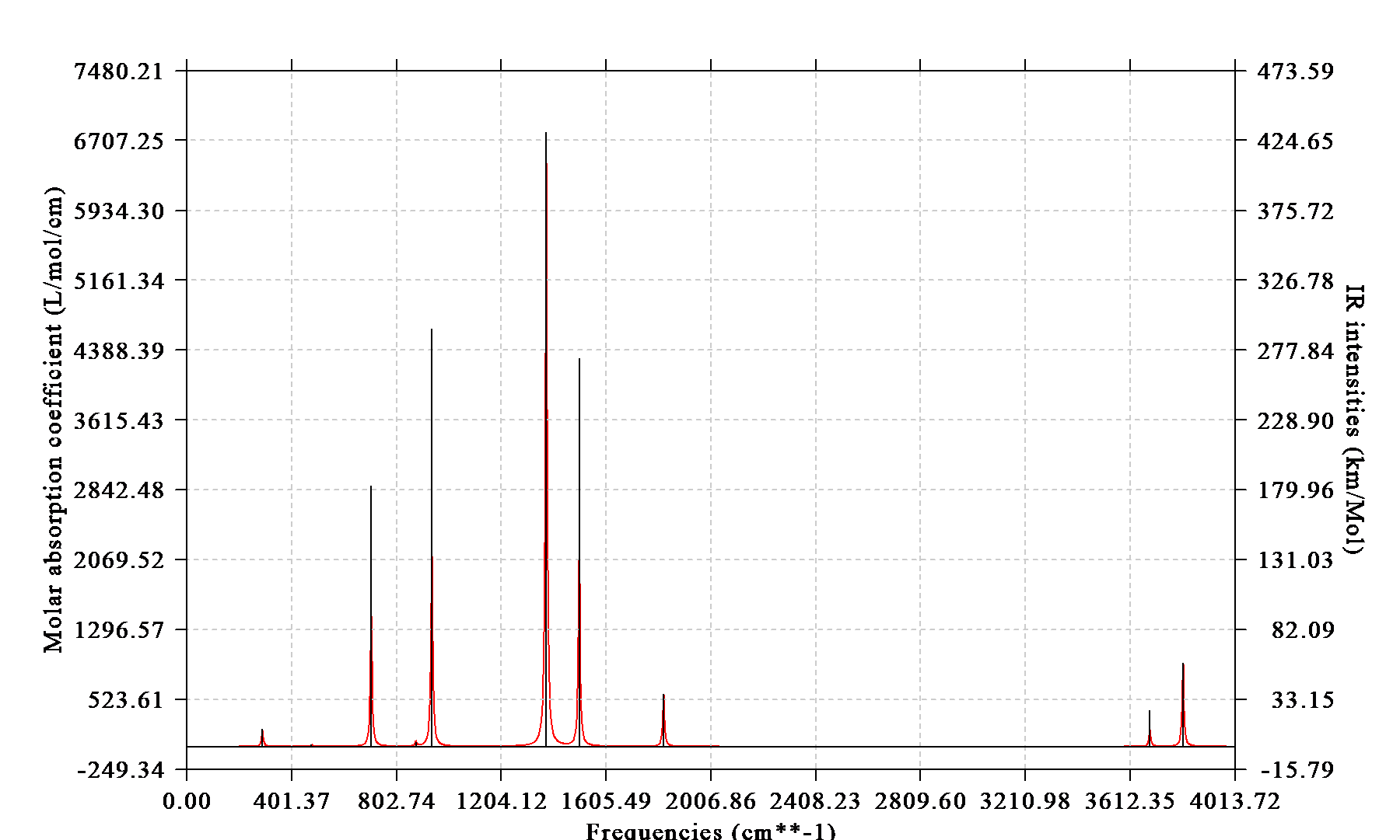
Below is an example of IR spectrum plotted by Multiwfn. Notice that the left axis corresponds to the curve (artificially broadened data), the right axis corresponds to the discrete lines (original transition data).

Example IR spectrum plotted by Multiwfn, with the broadened curve on the left axis and the discrete transitions on the right

Raman (normal or pre-resonance): Raman spectrum measures intensity of scattered light. Beware that for a specific vibration mode i, its Raman activity $S_{i}$ and Raman intensity $I_{i}$ are two different quantities. Raman activity is an intrinsic property of each molecular vibrational mode, while Raman intensity is directly related to experimental Raman spectrum, and its value is dependent on the choice of wavenumber of incident light ν₀ as well as temperature. The conversion relationship can be found in many papers, for example my paper Chem. Asian J., 16, 56 (2021) DOI: 10.1002/asia.202001228 gave it and you can cite:

\[I_i=\frac{C(\nu_0-\nu_i)^4S_i}{\nu_i B_i}\qquad B_i=1-\mathrm{exp}\left(-\frac{hc\nu_i}{kT}\right)\]

where C is a suitably chosen common normalization factor for all peak intensities, ν_i is vibrational frequency. Only the Raman spectrum broadened based on Raman intensities is strictly comparable to the experimental one; however, as the peak position of Raman activity and intensity are identical, and for a specific vibrational mode its intensity is proportional to its activity, the Raman spectrum broadened from Raman activities is also useful in some sense.

Almost all quantum chemistry codes only output Raman activities, therefore by default, Multiwfn emulates the Raman spectrum in terms of broadening Raman activities. However, you can also let Multiwfn to first convert the activities to intensities via option 19 ($v_{0}$ and T are provided by users) based on above formula, then the Raman spectrum will be obtained by broadening Raman intensities. The normalization coefficient C is fixed to 10^-12 in Multiwfn (which is unimportant since what we are interested in is the shape rather than the absolute height of Raman spectrum). The integral of the peak broadened by one unit of Raman activity or intensity is equal to 1.

UV-Vis: In theoretical chemistry field, oscillator strength (f) is used for representing the transition strength involved in UV-Vis spectrum, which is defined as

\[f_{ij}=\frac{2}{3}(E_j-E_i)\left|\unicode{x1D6CD}_{ij}\right|^2\]

where i and j stand for initial and final states, and they correspond to ground state and excited state in the context of UV-Vis spectrum, respectively. E is energy of state. |µ_ij|² is squared norm of transition electric dipole moment vector between the two states.

There is a relation between theoretical data and experimental spectra: If the unit 1000 c$m^{-1}$ and L/mol/cm are used for X-axis and Y-axis respectively, then the area under the curve that broadened from per unit f should be 1/4.32*10⁶. Equivalently, if eV is used as X-axis unit, the value should be 1/4.32/8.0655*10⁶=28700. Via this relation, UV-Vis spectrum can be simulated by theoretical data.

Fluorescence spectrum can also be plotted with exactly the same manner as UV-Vis, the only difference to UV-Vis is that according to Kasha's rule, you should only take the first singlet excited state (S1) into account, and geometry of optimized S1 state should be used (however, note that some systems break Kasha’s rule). For plotting phosphorescence spectrum, you should only take the first triplet excited state (T1) into account, and geometry of optimized T1 state should be used. Note that in order to obtain non-vanishing f corresponding to phosphorescence emission, spin-orbit coupling effect must be taken into account.

Directional UV-Vis: The |µ_ij|² mentioned above can be written as sum of its three Cartesian components, namely ${\left| {\unicode{x1D6CD}}_{ij} \right|}^{2}={\left( {\mu}_{ij}^{X} \right)}^{2}+{\left( {\mu}_{ij}^{Y} \right)}^{2}+{\left( {\mu}_{ij}^{Z} \right)}^{2}$. The so-called directional UV-Vis spectrum in Multiwfn refers to the case of only taking contribution of specific components of |µ_ij|² into account. You can choose to plot X, Y, Z, X+Y, X+Z, Y+Z or specific direction type of the spectrum. For example, if you plot X+Y type, then the ${\left| {\unicode{x1D6CD}}_{ij} \right|}^{2}$ will be replaced with ${\left( {\mu}_{ij}^{X} \right)}^{2}+{\left( {\mu}_{ij}^{Y} \right)}^{2}$, and the resulting spectrum will only exhibit the absorption due to interaction between present system and the electric field oscillating in X and Y directions. If you manually define the direction as (1,0,1), which corresponds to normalized vector of ($\frac{1}{\sqrt{2}},0,\frac{1}{\sqrt{2}}$), then ${\left| {\unicode{x1D6CD}}_{ij} \right|}^{2}={\left( {\frac{1}{\sqrt{2}}\mu}_{ij}^{X} \right)}^{2}+{\left( \frac{1}{\sqrt{2}}{\mu}_{ij}^{Z} \right)}^{2}$. Clearly, directional UV-Vis spectrum is very helpful in understanding the nature of optical absorption in terms of interaction with oscillating electric field of specific direction(s). In contrast, common UV-Vis spectrum corresponds to the case that the incident oscillating electric field is isotropic. Note that directional UV-Vis spectrum is additive, for example, sum of X and Y and Z types of the spectrum, and sum of X+Y and Z types of the spectrum, all equivalent to common UV-Vis spectrum.

ECD：The significance of rotatory strengths in ECD spectrum is analogous to oscillator strengths in UV-Vis spectrum, each electron transition mode corresponds to a rotatory strength. If the rotatory strengths are broadened, after somewhat scaling and shifting, the resultant curve will be comparable to experimental ECD spectrum. The integral of the peak broadened by one unit of rotatory strength is equal to 1. In quantum chemistry programs, such as Gaussian, rotatory strengths can be calculated in length representation or in velocity representation, in the former case the strengths are origin-dependent, while in the latter case the strengths are origin-independent. For complete basis set situation, the results in the two representations converge to the same values. Commonly, velocity representation is recommended to be used.

VCD: VCD measures difference in molecular absorption coefficient of left- and right-circularly polarized lights at different wavenumber λ, namely VCD curve can be expressed as $∆\varepsilon(\lambda)={\varepsilon}_{\mathrm{L}}(\lambda)-{\varepsilon}_{\mathrm{R}}(\lambda)$. Each vibrational mode has a rotatory strength, after broadening rotatory strengths of all vibrational modes, the shape of the resulting curve can be compared with experimental VCD spectrum. The integral area under the curve $∆\varepsilon(\lambda)$ contributed by a vibrational mode is proportional to its rotatory strength.

ROA: The ROA spectrum measures the difference between scattering intensity of right and left circularly polarized light:

\[\mathrm{ROA\ intensity}\equiv I_i^{\mathrm{R}}-I_i^{\mathrm{L}}\propto\frac{(\nu_0-\nu_i)^4A_i}{\nu_i B_i}\qquad B_i=1-\mathrm{exp}\left(-\frac{hc\nu_i}{kT}\right)\]

The ROA strength data outputted by Gaussian ROA task in fact is the $A_{i}$ term, which should be converted to actual ROA intensity according to above equation. The $A_{i}$ term is dependent on frequency of incident light. The integral of the peak broadened by one unit of ROA intensity/strength is equal to 1. There are several different forms of ROA, including ROA SCP(180), ROA SCP(90), ROA DCP(180). The 90 and 180 denote the angle between incident light and scattered light. The SCP (scattered circular polarization) means the incident light is linearly polarized light while the scattered light is circularly polarized light; DCP (dual circular polarization) corresponds to the case that both incident and scattered lights are circularly polarized light. The ROA SCP(180) is commonly employed, and it is also known as SCP backscattered ROA.

The ROA task of Gaussian also simultaneously outputs frequency-dependent Raman strength, which corresponds to the $R_{i}$ term of below equation

\[\mathrm{Raman\ intensity}\equiv I_i^{\mathrm{R}}+I_i^{\mathrm{L}}\propto\frac{(\nu_0-\nu_i)^4R_i}{\nu_i B_i}\qquad B_i=1-\mathrm{exp}\left(-\frac{hc\nu_i}{kT}\right)\]

correspondingly, there are also Raman SCP(180), Raman SCP(90) and Raman DCP(180) data. Since the current used incident light should be far from electron excitation energy, such Raman spectrum is called as far from resonance Raman.

3.13.2 Input file¶

Only the input files mentioned in this section are supported by Multiwfn for plotting spectrum purposes. DO NOT use such as .fch, .molden and .wfn as input file, evidently the data needed for plotting spectrum are not recorded in these files.

1 Gaussian output file¶

IR spectrum: Use output file of freq task as input. If you use Gaussian 09 D.01 or later revisions and meantime freq=anharm keyword was specified to carry out anharmonic analysis, Multiwfn will prompt you to choose if loading anharmonic frequencies and IR intensities instead of the harmonic ones.
Raman spectrum: Use output file of freq=raman task as input. If you would like to plot pre-resonance Raman spectrum, you should at the same time use CPHF=rdfreq keyword and write the frequencies of the incident lights after a blank line under the geometry specification, e.g. 300nm 400nm 500nm. If you hope to plot anharmonic Raman spectrum, use freq(raman,anharm) keywords, then Multiwfn will prompt you to choose if loading anharmonic frequencies and Raman activities instead of the harmonic ones.
VCD spectrum: Use output file of freq=VCD task as input. If you hope to plot anharmonic Raman spectrum (supported by Gaussian since G16), use freq(VCD,anharm) keywords, then Multiwfn will prompt you to choose if loading anharmonic frequencies and rotatory strengths instead of the harmonic ones.

For anharmonic IR, Raman and VCD spectra, you can choose if only loading anharmonic fundamental data, or simultaneously loading anharmonic overtone band or combination band data.
UV-Vis, directional UV-Vis and ECD spectrum: Use output file of TDDFT, TDHF, CIS, ZINDO or EOM-CCSD task as input, no additional keywords are required. The rotatory strengths in both length and velocity representation (the data under "R(length)" and "R(velocity)", respectively) can be chosen to be loaded by Multiwfn. Output file of optimization task for excited state can also be used, only the last output for transition information will be loaded by Multiwfn, therefore the resulting spectrum corresponds to final geometry.
ROA spectrum: Use output file of freq=ROA task as input. The frequencies of incident lights should be specified after a blank line under the geometry specification, e.g. 0.02, 0.03, 0.04, 0.05, the unit is default to a.u.; or write e.g. 500nm 520nm 550nm.

2 ORCA output file¶

IR spectrum: Use freq keyword.

Raman spectrum: Use keywords like below

! b3lyp def2-SVP numfreq
%elprop Polar 1 end

UV-Vis, directional UV-Vis and ECD spectrum: Commonly TDDFT is used, example of keywords:
```
! b3lyp def2-SVP
%tddft
nroots 20
TDA false
end
```
Notice that for TDDFT calculation, ORCA by default uses Tamm-Dancoff Approximation (TDA), in this case the oscillator strength and rotatory strengths are evidently not as good as those produced by TDDFT, therefore in the example above TDA false is used to make ORCA use standard TDDFT formalism. Also, it is worth noting that ORCA employs length representation for rotatory strengths in ECD.

Output file of sTDA or sTD-DFT task of ORCA (see below for details) is also supported by Multiwfn for plotting (directional) UV-Vis or ECD spectrum purpose. Below are example keywords:
```
! PBE0 def2-SVP def2/J RIJCOSX
%maxcore 6000
%pal nprocs 36 end
%tddft
Mode sTDDFT
Ethresh 10.0
maxcore 6000
end
```
Since ORCA 4.1 spin-orbit coupling (SOC) effect can be taken into account during TDDFT calculation, and all data needed for plotting SOC corrected UV-Vis and ECD spectra are automatically outputted. Therefore, when output file of SOC-TDDFT task is loaded into Multiwfn, when you enter UV-Vis and ECD plotting option, you can select if loading SOC corrected data instead of the one without SOC consideration. It is very easy to conduct SOC-TDDFT, simply adding dosoc true in %tddft section, for example:
```
%tddft nroots=40 TDA false dosoc true end
```
Output file of CIS, TDHF, ZINDO, EOM-CCSD, (DLPNO-)STEOM-CCSD calculations can also be used as input file for simulating (directional) UV-Vis and ECD spectra in Multiwfn.
VCD: Output file of regular frequency analysis task with %freq doVCD true end setting.
ROA spectra: Currently not supported by ORCA.

3 Grimme's sTDA output file¶

The sTDA proposed by Grimme in J. Chem. Phys., 138, 244104 (2013) is a method approximately solving the TDDFT equation and thus reduces the computational cost of the electron excitation part of TDDFT calculation by about two or three orders of magnitude. The corresponding sTDA program can be freely downloaded at https://github.com/grimme-lab/stda.

Although the Grimme's sTDA code has already been implanted into ORCA program, the tda.dat file outputted by standalone sTDA code can also be used as input file of Multiwfn for plotting UV-Vis or ECD purpose.

When ECD is to be plotted, you can choose which representation of rotatory strength will be used. The length and velocity representations have been mentioned above, while the mixed-form of representation, which is recommended in the sTDA original paper, is defined as $R_{M}$= $R_{V}$ × $f_{L}$ / $f_{V}$, where $f_{L}$ and $f_{V}$ are length and velocity representations of oscillator, respectively, and $R_{V}$ is the velocity representation of rotatory strength.

4 Grimme's xtb output file¶

The xtb program written by Grimme is mainly used to carry out GFN-xTB calculation (J. Chem. Theory Comput., 13, 1989 (2017) and J. Chem. Theory Comput., 15, 1652 (2019)), which may be viewed as a semiempirical variant of DFT method. It is not only robust but also rather fast, it can be conveniently applied to systems consisting of hundreds of atoms. Note that although the accuracy of xtb frequency has been verified to be basically reasonable, the quality of IR intensities outputted by xtb is not quite satisfactory (according to my experiences). xtb program can be freely obtained via https://github.com/grimme-lab/xtb/.

By running xtb test.xyz --ohesst, xtb will optimize the structure in test.xyz and then perform frequency analysis. The vibspectrum outputted in the current folder contains harmonic frequencies and IR intensities, it can be used as input file of Multiwfn for plotting IR spectrum purpose.

5 CP2K output file¶

Output file of vibrational analysis task of CP2K can be used as input file for plotting IR and Raman spectra. INTENSITIES T should present in &VIBRATIONAL_ANALYSIS. In addition, for plotting IR, the following content should present in &DFT:

    &PRINT
      &MOMENTS
        PERIODIC T  (for isolated systems, use F)
      &END
    &END

For plotting Raman spectrum, the following content should be presented in &FORCE_EVAL

  &PROPERTIES
    &LINRES
      PRECONDITIONER FULL_ALL
      &POLAR
        DO_RAMAN T
        PERIODIC_DIPOLE_OPERATOR T  (for isolated systems, use F)
      &END POLAR
    &END LINRES
  &END PROPERTIES

In addition, if you request CP2K to export .mol (Molden) file containing vibrational modes and IR intensities by adding the following content to &VIBRATIONAL_ANALYSIS field, then the .mol file can also be used as input file for plotting IR spectrum.

  &PRINT
    &MOLDEN_VIB
    &END MOLDEN_VIB
  &END PRINT

Output file of TDDFPT calculation of CP2K can be used as input file for plotting (directional) UV-Vis spectrum, and sTDA kernel is also supported. When spin-orbit coupling is activated by using following content in &TDDFPT section, then spin-orbit coupling corrected UV-Vis spectrum can be plotted.

      &SOC
      &END SOC
      &PRINT
        &SOC_PRINT
          SPLITTING
          SOME
        &END SOC_PRINT
      &END PRINT

X-adsorption spectrum may be plotted by Multiwfn based on .spectrum file produced by &XAS_TDP task of CP2K. You need to manually reorganize the data in the .spectrum to the plain text file, as shown below.

Note that CP2K input file of aforementioned tasks can be easily generated by corresponding option in subfunction 2 of main function 100.

6 BDF output file¶

Output file of TDDFT task of BDF can be used as input file for plotting UV-Vis spectrum.

7 Plain text file¶

For generality, Multiwfn supports plain text file as input, you can extract transition data from output files of computational chemistry packages other than the aforementioned ones, and then fill them into a file according to the format shown below

numdata inptype
energy strength [FWHM]                    ← For transition 1
energy strength [FWHM]                    ← For transition 2
energy strength [FWHM]                    ← For transition 3
...
energy strength [FWHM]                    ← For transition numdata

where numdata denotes how many entries are in this file. If inptype is set to 1, then only energy and strength will be read, and FWHMs for all transitions will be automatically set. If inptype is set to 2, then FWHMs will be read too. The transitions should be sorted according to the energies from low to high. The unit of both energy and FWHM should be in c$m^{-1}$ for IR, Raman, VCD and ROA spectra, in eV for UV-Vis and ECD spectra. The unit of strength should be in km/mol, Å⁴/amu, cgs (10^-40 erg-esu-cm/Gauss), 10^-44 es$u^{2}$ c$m^{2}$, 10⁴ K for IR, Raman, ECD, VCD, ROA spectra, respectively (oscillator strength of UV-Vis is dimensionless).

An example of the plain text file is shown below (for IR)

6 2
  81.32920        0.72170    8.0
 417.97970        3.58980    8.0
 544.67320       21.06430    8.0
 583.12940       41.33960    8.0
 678.66900       91.47940    8.0
 867.37410        2.94480    8.0

3.13.3 Usage and options¶

After booting up Multiwfn, first input path of output file of aforementioned programs or the plain text file containing transition data, then enter main function 11, and you will be asked to select the type of spectrum (for pre-resonance Raman and ROA, you also need to choose the frequency of interest), after that you will see below options. The meaning of some options may be different for various types of spectra.

Note that in this interface you can input s anytime to save current plotting settings to a file, or input l to load plotting settings from a file, so that you can quickly recover plotting status.

-4 Set format of saving graphical file: This is used to choose the format of the graphical file exported by option 1. Commonly, using vector formats such as ps, pdf and svg is recommended.

-2 Export transition data to plain text file: Output energies, intensities and FWHMs of all transitions to transinfo.txt in current directory, this file fully complies with the format introduced in last section, so it can be directly used as input file.

-1 Show transition data: Print energy and intensity data of all transitions on screen.

0 Plot spectrum: Plot spectrum right now! The spectrum will be shown on screen, and meantime the minima and maxima of the spectrum curve will be shown in console window.

1 Save graphical file of the spectrum in current folder: As the title says.

2 Export X-Y data set of lines and curves to plain text file: Export X-Y data set of lines and broadened spectrum to spectrum_line.txt and spectrum_curve.txt in current directory, respectively, you can replot the curve and discrete line graph directly by the two files via external program, such as Origin.

3 Set lower and upper limit of X-axis: As the title says. The interval between ticks also needs to be inputted. By default, the range of X-axis is adjusted automatically according to minimum and maximum transition energies.

4 Set left Y-axis: Set starting value, ending value and step size for left Y-axis. By default, the range of Y-axis is adjusted automatically according to the maximum peak.

5 Set right Y-axis: Like option 4, but for right Y-axis.

In many cases, after you adjust setting for Y-axis at one side, the position of zero point of this Y-axis deviates from that of Y-axis at another side, which makes the graph weird; To address this problem, options 4 and 5 enable you to choose if correspondingly adjusting range of Y-axis at another side. If you input y, then lower/upper limit and label interval of Y-axis at another side will be proportionally scaled to make zero point of left and right Y-axes are in the same horizontal line.

6 Select broadening function: Gaussian, Lorentzian and Pseudo-Voigt function can be selected for broadening discrete lines as curves.

7 Set scale ratio for curve: If the value is set to k, then the height of curve will multiply k in full range. For Raman, ECD, VCD and ROA spectra the default value is 1.0, for IR the value is 100, for UV-Vis spectrum an empirical value 28700.0 is used when energy unit is eV or nm, when unit is 1000 c$m^{-1}$ the value 1/(4.32*10^-6) is used.

8 Input full width at half maximum (FWHM): As the title says.

9 Toggle showing discrete lines: Choose if show the discrete lines corresponding to transitions on the spectrum graph.

10 Switch the unit of infrared intensity / Set the unit of excitation energy: For IR spectrum, switch the unit of IR intensities between km/mol (default) and es$u^{2}$*c$m^{2}$. For UV-Vis and ECD spectra, choose the unit of energy between eV, nm and 1000 c$m^{-1}$.

11 Set Gaussian-weighting coefficient: Sets $w_{\mathrm{gauss}}$, which is mentioned in Section 3.12.1, this option only appears when Pseudo-Voigt function is chosen.

12 Set shift value in X: If the value is set to k, then the final curve and discrete lines will be shifted by k in X direction.

13 Set colors of curve and discrete lines: As the title says.

14 Set scale factor for transition energies (or vibrational frequencies): Using this option, transition energies can be scaled by a factor, the spectrum to be plotted will be affected.

For scaling vibrational frequencies, there are two methods that can be used:

(1) Uniform scaling: The selected frequencies are simply multiplied by a factor inputted by the user. You can choose the frequencies according to their index range or frequency range.
(2) Power-law scaling: This method was proposed in J. Chem. Theory Comput. (2026) DOI: 10.1021/acs.jctc.6c01138, it performs better than the uniform scaling. Every frequency is scaled as ${\lambda}_{1}{\omega}^{{\lambda}_{2}}$, where λ₁ and λ₂ are fitted parameters specified by the user and ω is the original frequency.

15 Output contributions of individual transitions to the spectrum: If select this option, user will be prompted to input a criterion (e.g. k), then not only the total spectrum (as option 2), but also the contributions from the individual transitions whose absolute value of strength larger than k will be outputted to spectrum_curve.txt in current folder. This feature is particularly useful for identifying the nature of total spectrum.

In this function you can also input 0 first, then input an X position of the spectrum, then 10 transitions having largest contribution to this position will be shown, this is quite convenient to make clear major contributors at specific spectrum positions (e.g. peak positions of important absorptions).

16 Set status of showing labels of spectrum minima and maxima: You will enter an interface, in which there are many options used to set how to show spectrum minima and maxima on the plotted map, they are self-explanatory.

17 Other plotting settings: Miscellaneous plotting settings can be set here, such as if showing dashed grid lines, if showing labels on axes, text size of axis name / ticks / legends, number of decimal places in axes, type of labels in left Y-axis, position of legends, set color of line and curve of different systems.

18 Toggle weighting spectrum of each system: See explanation in next section.

19 Convert Raman (or ROA) activities to intensities: As mentioned earlier, this option is used to convert Raman (or ROA) activities to intensities. After that, the Raman (or ROA) spectrum plotted by option 0 will be the one broadened based on Raman (or ROA) intensities rather than Raman (or ROA) activities. The wavenumber of incident light and temperature are inputted by users.

20 Modify strengths: You can select some transitions and change their strengths (depending on spectrum type) to specific value. This option is very useful if you would like to plot fluorescence spectrum, in this case you need to set oscillator strength of all transitions except for the lowest singlet excitation to zero (Kasha's rule).

21 Set status of showing weighted curve and curves of individual systems: As shown in the next section, Multiwfn is able to plot weighted spectrum according to given weights of multiple systems. This option controls if plotting weighted curves and curves of various systems.

22 Set thickness of curves/lines/texts/axes: As the title says.

23 Set status of showing spikes to indicate transition levels: Via this option, you can plot one or multiple sets of spikes at bottom of the spectrum to indicate position of different sets of transitions. If some transitions are degenerated, the height of spikes can be used to reflect degree of degeneracy. See Section 4.11.9 for illustration of this option. This option is not available when multiple systems are considered in the plotting simultaneously.

Note that the actual number of points constituting the spectrum is controlled by "num1Dpoints" parameter in settings.ini. The default value is commonly large enough and thus need not to be adjusted.

3.13.4 Plotting multiple systems together and weighted spectrum¶

In Multiwfn, it is possible to simultaneously plot spectrum for multiple files, and meantime taking weights into account. This feature is quite useful for obtaining actual spectrum of a flexible molecule with many thermally accessible conformations.

For example, there is a molecule containing four accessible conformations, their distribution ratio has been determined according to Boltzmann's method based on calculated free energies. If you want to plot its weighted spectrum and spectrum of each conformation, you should write a plain text file named multiple.txt (other file name cannot be recognized by Multiwfn), the content is:

boltz\Excit\a.out 0.6046
boltz\Excit\b.out 0.1950
boltz\Excit\c.out 0.1686
boltz\Excit\d.out 0.0317

where the first and second column correspond to path of input file and weight of each conformation. Different types of input file can be presented together in this file. If you use this file as input file, after you entered spectrum plotting module, Multiwfn will load data from these files in turn. When plotting spectrum, spectrum of all the four conformations will be separately calculated and drawn with different colors. In addition, the weighted spectrum is plotted on the graph as thick red curve, it is simply evaluated as follows:

weighted spectrum = 0.6046×a + 0.1950×b + 0.1686×c + 0.0317×d

In the graph you can also observe many black discrete lines, these are collection of discrete lines corresponding to different conformations. Notice that their heights have already been multiplied by corresponding weights.

If before plotting spectrum you have chosen option 18 once, then the spectrum of various conformations shown on graph are the weighted ones; in other words, these curves represent contribution of each conformation to actual spectrum (thick red curve). In this case, the color of weighted discrete lines is no longer all black but in accordance with color of curves, so that users can easily recognize correspondence between curve and discrete among different systems.

If you simply want to simultaneously plot spectrum for multiple systems but do not want to draw weighted spectrum, then the second column of multiple.txt should not be weights, but customized legends, for example

boltz\Excit\a.out Molecule A
boltz\Excit\b.out Molecule B
boltz\Excit\c.out Molecule C
boltz\Excit\d.out Molecule D

Then plot spectrum as usual, curve of all the four systems will be shown together, and the legends will be "Molecule A", "Molecule B", etc.

Note

When the legend is completely composed of numbers, the legend will be regarded as weight. If the legends have to be a number, you should add $ in front of the legend to let Multiwfn know it is legend rather than weight. For example, $50 will be recognized as legend of “50”.

If you are using Linux platform and some file paths in the multiple.txt contains / symbol or space, you should add double quotation marks at the two ends of the file path, so that the path could be properly loaded.

3.13.5 Plotting NMR spectrum¶

Theory¶

Many quantum chemistry programs are able to compute magnetic shielding tensors σ at nuclei, usually only the average of its diagonal terms, namely isotropic magnetic shielding value σ_iso, is of interest, because NMR spectrum is commonly determined in solvent environment and the solute is able to freely rotate.

The chemical shift δ is calculated as follows

\[\delta=\frac{\sigma^{\mathrm{ref}}-\sigma}{1-\sigma^{\mathrm{ref}}}\approx\sigma^{\mathrm{ref}}-\sigma\]

where σ^ref is shielding value of reference substance (tetramethylsilane for ¹³C and ¹H NMR), while the σ is shielding value of the sample to be determined. The two values should be evaluated at exactly the same calculation setting (theoretical method, basis set, solvation model...).

Another way of determining chemical shift is scaling method, see http://cheshirenmr.info for detail. Briefly speaking, this method evaluates δ in a very simple way:

\[\delta=a\times\sigma+b\]

where the a and b are prefitted slope and intercept parameters based on a training set for specific calculation level. For example, if the optimization is conducted under vacuum using B3LYP/6-31G* while shielding value is calculated using B3LYP/6-31G* under chloroform environment represented by SMD solvation model, then a = -1.0157 and b = 32.2109 for ¹H NMR, while a = -0.9449 and b = 188.4418 for ¹³C NMR.

If there are methyl groups in the system, the δ of its three hydrogens should be averaged before generating NMR spectrum, since methyl groups can freely rotate in actual environment due to its extremely low rotation barrier. In addition, if there are multiple thermally accessible conformers and they can interconvert with each other easily, the weighted average shielding value should be calculated for each atom based on weights of the conformers:

\[\overline{\delta^A}=\sum_i p_i\delta_i^A\]

where i is conformer index and A is atom index. $p_{i}$ stands for weight of conformer i, which can be calculated according to Boltzmann distribution based on relative free energies between the conformers.

With δ of all atoms in hand, one can plot discrete line map of NMR, the X-axis of the spikes in the map corresponds to δ while Y-axis corresponds to degeneracy, which is N if maximal spacing between N chemical shifts is less than specific threshold (e.g. 0.05 ppm), for other cases the degeneracy is 1.0.

Actual NMR spectrum with finite peak width can be generated by broadening the spikes by Lorentzian function, the full width at half maximum (FWHM) is a key parameter of controlling peak shape. In this curve map, the peak height corresponds to strength of NMR signal.

Input file¶

Output file of NMR task of Gaussian, ORCA and BDF programs are directly supported as input file for plotting NMR spectrum. .data file generated by NMR task of CP2K can also be used.

Example of NMR task of Gaussian

# B972/def2tzvp scrf=solvent=chloroform NMR

Title Card Required

0 1
 N                 -0.14557000    1.69364200    0.17479300
 H                 -1.18363600    1.59873700    0.51496300
[...ignored]

Example of NMR task of ORCA

! B3LYP/G 6-31G* NMR cpcm(chloroform) RIJK autoaux
* xyz   0   1
 C                     0.        1.14218   0.72212
 C                     0.        1.19872  -0.67302
[...ignored]

Example of NMR task of CP2K. Adding the following content into &FORCE_EVAL of input file of a common GAPW task. In addition, it is suggested to set &SCF / EPS_SCF to 1E-7 and EPS_DEFAULT to 1E-14 to guarantee sufficient numerical accuracy.

&LINRES
  PRECONDITIONER FULL_KINETIC
  EPS 1E-8
  MAX_ITER 300
  &CURRENT
    CHI_PBC T
    GAUGE R_AND_STEP_FUNCTION
    ORBITAL_CENTER ATOM
  &END CURRENT
  &LOCALIZE
     MAX_ITER 20000
     EPS_LOCALIZATION 1E-5
  &END LOCALIZE
  &NMR
  &END NMR
&END LINRES

Plain text file

Plain text file recording atom names and shielding values can also be used as input file for plotting NMR spectrum, see examples\spectra\NMR\general.txt for example. Thus in principle Multiwfn can plot NMR for any program that can yield shielding values.

Usage¶

After loading input file, entering main function 11 and selecting NMR, you will see the NMR plotting interface. Then if you select option 0, NMR spectrum will be displayed, and raw data will be shown on console window. Since most options in this interface are self-explanatory, only a few noteworthy options are mentioned below.

-2 Export NMR data to a plain text file: This option exports shielding values to NMRdata.txt in current folder. If you have used option 7 to convert shielding values to chemical shifts, then both of them will be exported.
6 Choose the element considered in plotting: Via this option you can choose the element to be considered. For example, if you want to plot ¹H NMR spectrum or examine relevant data, you should select this option and input H.
7 Set how to determine chemical shifts: By default, the X-axis in the plotted NMR spectrum corresponds to magnetic shielding value, while if want to make chemical shift δ as X-axis, you should select this option prior to plotting. In this option you can select the way of determining δ:

(1) Taking difference between shielding value of current system and reference system. You can manually input reference value or directly use built-in data.

(2) Using scaling method to determine the δ. You can manually input the fitted slope and intercept, or directly use built-in data.

There are several sets of built-in data, they correspond to the levels very suitable for calculating δ.
10 Average shielding values of specific atoms: For example, usually the δ of the hydrogens in the same methyl group should be averaged, you can use this function to realize this purpose.
11 Set strength of specific atoms: By default, every atom has strength of 1.0, namely contributes to degeneracy by 1.0. You can use this option to modify strength of specific atoms. For example, if you set strength of atoms 3, 6, 7 to 0, then these atoms will disappear in the plotted spectrum.
16 Change setting of labelling atoms: In order to distinguish the atoms in the NMR spectrum, Multiwfn labels atomic indices on the plotted peaks. You can use this option to control details of labelling, such as position, size, color, content of the labels and so on.

Plotting conformation weighted spectrum and spectrum containing multiple systems¶

Conformation weighted NMR spectrum can be plotted by using plain text file as input (the name must contain "multiple", for example, valine_multiple.txt is a valid name), each line contains path of an input file and corresponding conformation weight, for example:

D:\valine\conf1.out 0.43
D:\valine\conf2.out 0.25
D:\valine\conf3.out 0.32

If you simply want to plot NMR spectrum of multiple systems together, specifying file path and legend in each line, for example

/lovelive/nico.out Isomer 1
/lovelive/nozomi.out Isomer 2

Then after entering NMR plotting interface, you can plot the spectrum via exactly the same steps as plotting single system. Note that all systems must have the same number of atoms.

Special notes¶

To save the NMR spectrum as graphical file, you can choose option 1. It is highly suggested to use pdf format, because it is a vectorial format, the spectrum can be losslessly zoomed in and out, and the lines and texts look very smooth. The format can be chosen by option -3, and the default format can be changed by "graphformat" in settings.ini.

After adjusting various plotting settings, you can input s in the interface to save plotting settings to a specific text file, so that when you want to replot the NMR spectrum with exactly the same effect in the future, you can input l to directly restore plotting settings from the text file. Note that any operation on plotted data must be manually redone every time (e.g. averaging shielding values, converting shielding values to chemical shifts, etc.).

Some examples of plotting NMR spectrum are given in Section 4.11.10.

3.13.6 Partial vibrational spectrum (PVS) and partial vibrational density-of-states (PVDOS)¶

The partial vibrational spectrum (PVS) was proposed by me to intuitively understand nature of peaks of vibrational spectra. Partial vibrational density-of-states (PVDOS) is closely related to it. In this section I will describe their definition and implementation in Multiwfn.

3.13.6.1 Theory¶

PVS and PVDOS¶

Recall that vibrational spectrum curve can be represented as follows

\[\varepsilon(E)=c\sum_i f_i G(E-E_i^{\mathrm{vib}})\]

where c is a constant depending on type of vibrational spectrum, i loops over all vibrational modes, f and $E^{\mathrm{vib}}$ respectively correspond to strength (e.g. IR intensity for IR spectrum, rotatory strength for VCD spectrum) and transition energy of a vibration mode, and G is broadening function (usually Lorentzian function for vibrational spectrum).

PVS method decomposes the total vibrational spectrum as contributions from different fragments. The PVS curve of fragment A is expressed as

\[\varepsilon_A(E)=c\sum_i\Theta_A^i f_i G(E-E_i^{\mathrm{vib}})\]

where ${\Theta}_{A}^{i}$ is composition of fragment A in vibrational mode i.

Vibrational density-of-states (VDOS) represents density of vibrational transitions per wavenumber, which is represented as

\[\rho(E)=c\sum_i G(E-E_i^{\mathrm{vib}})\]

The coefficient c and the unit of VDOS are arbitrary, only relative magnitude of VDOS at different energies is of interest. The partial VDOS (PVDOS) curve of fragment A is expressed as

\[\rho_A(E)=c\sum_i\Theta_A^i G(E-E_i^{\mathrm{vib}})\]

Type of fragment¶

In Multiwfn, maximally 10 fragments can be defined simultaneously to draw their PVS or PVDOS curves. The fragment(s) can be defined in two ways:

(1) A set of atoms. Their all Cartesian coordinates or specific Cartesian components (i.e. X, Y, Z, XY, XZ, or YZ) can be taken into account.

(2) A set of redundant internal coordinates (RIC). The RICs may be bonds, angles and dihedrals, and they are allowed to be mixed in a fragment.

Composition of fragment in vibrational modes¶

The way of calculating ${\Theta}_{A}^{i}$ is not unique. Each vibration mode has two key characters, normal coordinate and intensity, so ${\Theta}_{A}^{i}$ can be defined as percentage contribution of fragment A to either of them of vibrational mode i, as described below.

Composition type 1: Percentage contribution to normal coordinate

Normal coordinate q of each vibrational mode represents motion of 3$N_{\mathrm{atom}}$ atomic Cartesian coordinates {x} involved in the vibration. Let $L_{j}$_,_i represent component of $x_{j}$ in $q_{i}$, and assume that $q_{i}$ is normalized, then ${\Theta}_{A}^{i}$ is defined as

\[\Theta_A^i=100\%\times\sum_{j\in A}L_{j,i}^2\]

where j loops over all or specific Cartesian coordinates of atoms in fragment A.

Composition type 2: Percentage contribution to intensity

This type of composition is much more complicated than the composition type 1, and currently is only applicable to IR intensity. IR intensity of vibrational mode i is expressed as

\[I^i=s\left|\frac{\partial\unicode{x1D6CD}}{\partial q_i}\right|^2=s\sum_{\sigma=x,y,z}\left(\frac{\partial\mu_\sigma}{\partial q_i}\right)^2\]

where s is a constant factor, and µ_σ stands for Cartesian component σ of electric dipole moment of present system. The derivative of µ_σ with respect to $q_{i}$ can be further written as sum of product of dipole moment derivative to atomic Cartesian coordinates and corresponding components of normal coordinates:

\[\frac{\partial\mu_\sigma}{\partial q_i}=\sum_j\frac{\partial\mu_\sigma}{\partial x_j}\frac{\partial x_j}{\partial q_i}\equiv\sum_j\frac{\partial\mu_\sigma}{\partial x_j}L_{j,i}\]

After a simple arrangement, IR intensity can be expressed as follows, where fragment B contains all atomic Cartesian coordinates that do not belong to fragment A

\[I^i=s\sum_{\sigma=x,y,z}\left[I_{A,\mathrm{intra}}^{i,\sigma}+I_{B,\mathrm{intra}}^{i,\sigma}+I_{AB}^{i,\sigma}\right]\]

where

\[\begin{gathered}I_{A,\mathrm{intra}}^{i,\sigma}=\left(\sum_{j\in A}\frac{\partial\mu_\sigma}{\partial x_j}L_{j,i}\right)^2\qquad I_{B,\mathrm{intra}}^{i,\sigma}=\left(\sum_{k\in B}\frac{\partial\mu_\sigma}{\partial x_k}L_{k,i}\right)^2\\ I_{AB}^{i,\sigma}=2\left(\sum_{j\in A}\frac{\partial\mu_\sigma}{\partial x_j}L_{j,i}\right)\left(\sum_{k\in B}\frac{\partial\mu_\sigma}{\partial x_k}L_{k,i}\right)\end{gathered}\]

in which ${I}_{A,\mathrm{intra}}^{i,\sigma}$ stands for intrafragment contribution of fragment A to mode i in σ direction, and ${I}_{A\mathrm{B}}^{i,\sigma}$ corresponds to contribution from coupling of fragments A and B. There is no unique way to partition the coupling term to the fragments, I prefer to simply equally dissect it, in this case contribution of fragment A to $I^{i}$ is written as

\[I_A^i=s\sum_{\sigma=x,y,z}\left(I_{A,\mathrm{intra}}^{i,\sigma}+\frac{1}{2}I_{AB}^{i,\sigma}\right)=s\sum_{\sigma=x,y,z}\left(\sum_{j\in A}\frac{\partial\mu_\sigma}{\partial x_j}L_{j,i}\right)\left(\sum_k\frac{\partial\mu_\sigma}{\partial x_k}L_{k,i}\right)\]

Finally, ${\Theta}_{A}^{i}$ is calculated as

\[\Theta_A^i=100\%\times\frac{I_A^i}{I^i}\]

Note that the ${\Theta}_{A}^{i}$ defined in above way could be slightly negative or larger than 100% in some cases, this is unavoidable and never means the result is incorrect. Negative value comes from the fact that the interfragment coupling contribution may be negative, whose magnitude can even be greater than the positive intrafragment contribution.

Summary of type of fragment spectrum¶

Taking all information described above, now we can define different forms of spectrum representing fragment contribution to vibration modes, the following ones are currently supported in Multiwfn:

PVS-NC(atom)
PVS-NC(RIC)
PVS-I(atom)
PVDOS-NC(atom)
PVDOS-NC(RIC)

The meaning of PVS and PVDOS is clear. “I” and “NC” mean that the composition of fragment in a vibrational mode are defined as fragment contribution to its intensity and normal coordinate, respectively. (atom) and (RIC) denote that the fragments are composed of a set of atoms (and maybe some of their Cartesian components) and redundant internal coordinates, respectively.

As mentioned earlier, PVS-I(atom) can only be used for decomposition analysis of IR spectrum, while PVS-NC(atom/RIC) can be used to decompose any kind of vibrational spectrum. PVDOS is independent of type of vibrational spectrum, because it does not involve strength information.

Different types of spectra have different practical values. For example, from PVS-NC(atom) you can intuitively recognize which atoms mainly participate in active vibration modes in different wavenumber ranges, while PVS-NC(RIC) allows you to study this in terms of internal coordinate motions. Via PVS-I(atom), you can vividly understand which atomic motions in vibrations make a notable contribution to IR absorption intensity at different wavenumbers. Spectral inactive vibrational modes cannot be visually studied by means of PVS-NC or PVS-I spectra, however, one can respectively utilize PVDOS-NC(atom) and PVDOS-NC(RIC) to easily understand which atoms and internal coordinates are significantly involved in vibration modes lying in different energy regions.

Overlap PVS (OPVS) and overlap PVDOS (OPVDOS)¶

In order to visually study coupling effect of atomic motions of different two fragments in vibrational spectrum, I defined OPVS and OPVDOS, which are respectively expressed as

\[\begin{gathered}\varepsilon_{AB}(E)=c\sum_i\Theta_{AB}^i f_i G(E-E_i^{\mathrm{vib}})\\ \rho_{AB}(E)=c\sum_i\Theta_{AB}^i G(E-E_i^{\mathrm{vib}})\end{gathered}\]

where A and B are the two fragments for which you want to study their coupling effect, ${\Theta}_{AB}^{i}$ is their percentage coupling contribution to vibrational mode i.

For overlap PVS-NC (OPVS-NC) and overlap PVDOS-NC (OPVDOS-NC), ${\Theta}_{AB}^{i}$ is defined as

\[\Theta_{AB}^i=100\%\times 2\times\mathrm{min}(\Theta_A^i,\Theta_B^i)\]

If mode i is equally contributed by fragments A and B, namely ${\Theta}_{A}^{i}={\Theta}_{B}^{i}=50\%$, then ${\Theta}_{AB}^{i}=100\%$. At a wavenumber, the closer the OPVS-NC (${\varepsilon}_{AB}$) curve to ε curve, or the close the OPVDOS-NC (${\rho}_{AB}$) curve to ρ curve, the more the spectrum at this wavenumber exhibits the collective motion of fragments A and B.

For overlap PVS-I (OPVS-I) spectrum, ${\Theta}_{AB}^{i}$ is defined as $100\%\times {I}_{AB}^{i}/{I}^{i}$, where ${I}_{AB}^{i}$ is coupling contribution of fragments A and B to vibration mode i:

\[I_{AB}^i=s\sum_{\sigma=x,y,z}I_{AB}^{i,\sigma}\]

The more positive (negative) the OPVS-I curve, the more the IR absorption is enhanced (suppressed) by the interfragment coupling effect.

3.13.6.2 Usage¶

To plot the spectrum curves contributed by fragments introduced above, after booting up Multiwfn, you need to load input file for plotting common vibrational spectrum, then enter main function 11, select the type of the vibrational spectrum you want to plot, including IR, Raman, VCD or ROA (PVS-I only supports IR. For VDOS, all of them are equivalent). Then, after choosing option “24 Set partial vibrational spectra (PVS) or vibrational DOS (VDOS)”, you will enter an interface for defining fragments and adjusting relevant plotting settings. As you can see from screen, by inputting t, you can select the type of the fragment spectrum. By inputting a number, you can define the fragment with that index, please carefully follow the prompts on screen, at most 10 fragments can be defined. If you have defined two or more fragments, you can then use option 0 to choose two fragments for which the OPVS or OPVDOS curve will be plotted.

Once defining fragments has finished, you can input q to leave the interface, and at the same time, Multiwfn will load needed data from input file and generate composition of various fragments in every vibrational mode, and the quantitative result will be shown on screen. (For PVS-I, you will also be asked to input the .fch/fchk file produced by “freq” task of Gaussian, from which Multiwfn will load data needed for calculating IR intensities. At the same time, Multiwfn asks you if outputting IRinten.txt file, which contains very detailed raw and intermediate information about IR intensity evaluation, which is particularly helpful for you to understand source of ${I}_{A}^{i,\sigma}$)

After leaving option 24, you can plot vibrational spectrum as usual by choosing option 0, the PVS/OPVS or VDOS/OPVDOS curves will be displayed together with vibrational spectrum curve.

Note that for plotting Raman or ROA spectrum together with accompanied PVS-NC curves, you need to convert Raman activities to Raman intensities first as usual.

Input file¶

PVS-NC(atom) and PVDOS-NC(atom): You can use output file of frequency analysis of Gaussian, ORCA, and CP2K programs as input file.

xtb program is also supported but the situation is slightly special: After performing Hessian calculation task by xtb, you will have vibspectrum and g98.out files. After booting up Multiwfn you should load the vibspectrum, and after defining fragments and leaving the interface of option 24, you will be asked to input the path of the g98.out, from which Multiwfn will load normal coordinates.
PVS-NC(RIC) and PVDOS-NC(RIC): You should use output file of frequency analysis of Gaussian as input file. freq=intmodes keyword of Gaussian must be used, so that composition of RICs in various vibrational modes will be written to Gaussian output file, which will be loaded by Multiwfn when leaving option 24.
PVS-I(atom): You should use output file of frequency analysis of Gaussian as input file, and the .fch/fchk file converted from the .chk file produced by this task must be kept, which is requested to be provided by Multiwfn when leaving option 24.

Examples of plotting (O)PVS and (O)VDOS are given in Section 4.11.12.

3.13.7 Predicting color based on UV-Vis spectrum curve¶

Multiwfn provides a very useful and powerful function to predict color of a chemical substance based on its UV-Vis adsorption spectrum curve. Very detailed explanation can be found in my blog article “Predicting color of chemical substances through quantum chemistry calculations and Multiwfn program” (http://sobereva.com/662, in Chinese), here only key information is given.

Theory¶

A chemical substance displays a color if it has optical adsorption in visible light range, and the displayed color corresponds to the reflection and transmission lights. Essentially, the displayed color is the complementary color with respect to the color corresponding to the UV-Vis adsorption spectrum (i.e. adsorption color). In order to convert the UV-Vis spectrum to the displayed color, the following steps are needed:

(1) Calculate X, Y, Z values of CIE1931 XYZ color space based on CIE1931 2° tristimulus functions (tabulated data given in literature) and the UV-Vis spectrum generated in usual way. See https://www.oceanopticsbook.info/view/photometry-and-visibility/chromaticity for details.
(2) Convert X, Y, Z values to R, G, B values of sRGB color space via linear transformation. See https://www.oceanopticsbook.info/view/photometry-and-visibility/from-xyz-to-rgb for details. Note that Gamma correction is not used.
(3) If any of R, G, B values exceeds valid range of sRGB color space, scale it into valid range, namely [0,1].
(4) Take complementary color of the color corresponding to the adsorption light as (1.0-R,1.0-G,1.0-B).
(5) Obtain maximum brightness colors of the adsorption color and its complementary color by respectively shifting their maximum components to 1.0, so that the two colors have equal brightness.

Now, the maximum brightness of complementary color can be regarded as the color actually displayed by the chemical substance.

Note that Multiwfn not only reports R, G, B components of adsorption color and complementary color in [0,1], but also reports in [0,255] range.

Usage¶

There are two ways of using Multiwfn to predict color

Case 1: Predicting color directly based on the theoretical UV-Vis spectrum generated by Multiwfn

In this case, the input file is the same as that for plotting UV-Vis spectrum as described in Section 3.13.2. After loading input file, enter main function 11, select option “25 Evaluate color based on the spectrum in visible range”, then UV-Vis spectrum within 360-830 nm will be first shown on screen, after closing it, you will see adsorption color corresponding the UV-Vis spectrum and its complementary color. At the same time, maximum brightness forms of these two colors are also shown on screen. Commonly the color shown at bottom right corner of the window can be regarded as the actually displayed color of the substance. Meantime, from command-line window of Multiwfn, you can find detailed parameters of the colors shown on screen, such as CIE1931 XYZ values, RGB values in sRGB color space, etc.
Case 2: Predicting color for a given spectrum curve recorded in plain text file

In this case, you can predict color based on e.g. experimentally determined spectrum curve. The input file should be a plain text file containing two column data, the first column is wavelength in nm, the second column is absorbance in arbitrary unit (see examples\spectra\Allura_red_UV-Vis.txt for example. The data range and spacing are arbitrary, the two columns should be separated by space or comma). After loading the input file, enter main function 11 and then choose option “0: Predicting color based on UV-Vis spectrum recorded in text file”, you will see predicted colors, the information provided by Multiwfn has the same form as that mentioned in case (1).

Two noteworthy points¶

The present function evidently can also be used to predict color of emission spectrum. For example, there is a system satisfying Kasha’s rule. To predict its fluorescence spectrum, you should perform electron excitation calculation at its optimized S1 geometry, and use the output file as input file of Multiwfn. After entering main function 11 and selection option 3 to enter the module for plotting UV-Vis spectrum, you should first select option “20 Modify oscillator strengths” to set oscillator strength of all excited states except for S1 to zero, and then use option 25 to predict color of the present spectrum (corresponding to fluorescence spectrum). In this case you should take the color shown under “color” label on the graphic window as the color of fluorescence emission, and the complementary color shown on the window is useless in this case.

Flexible molecules often have multiple conformations with nonnegligible weight at the temperature of interest, if some of them show distinctly different light adsorption character in visible light range, to reliably predict color you must take conformation weighting average of spectrum into account. You should use multiple.txt containing weights of the conformations (see Section 3.13.4) as input file of Multiwfn in this case, and then predict color via regular steps mentioned above.

Examples of predicting colors can be found in Section 4.11.14.