4.3 Output and plot various properties in a line

4.3.1 Plot the spin density curve of triplet formamide along carbon and oxygen atoms

Boot up Multiwfn and input following commands

examples\formamide-m3.wfn
3  // Main function 3, plot real space function along a line
5  // Spin density
1  // Defining the line by nuclear coordinate of two atoms
1,6  // Indices of the two atoms, carbon and oxygen atoms correspond to 1 and 6 in present example, respectively

The graph shows up immediately:

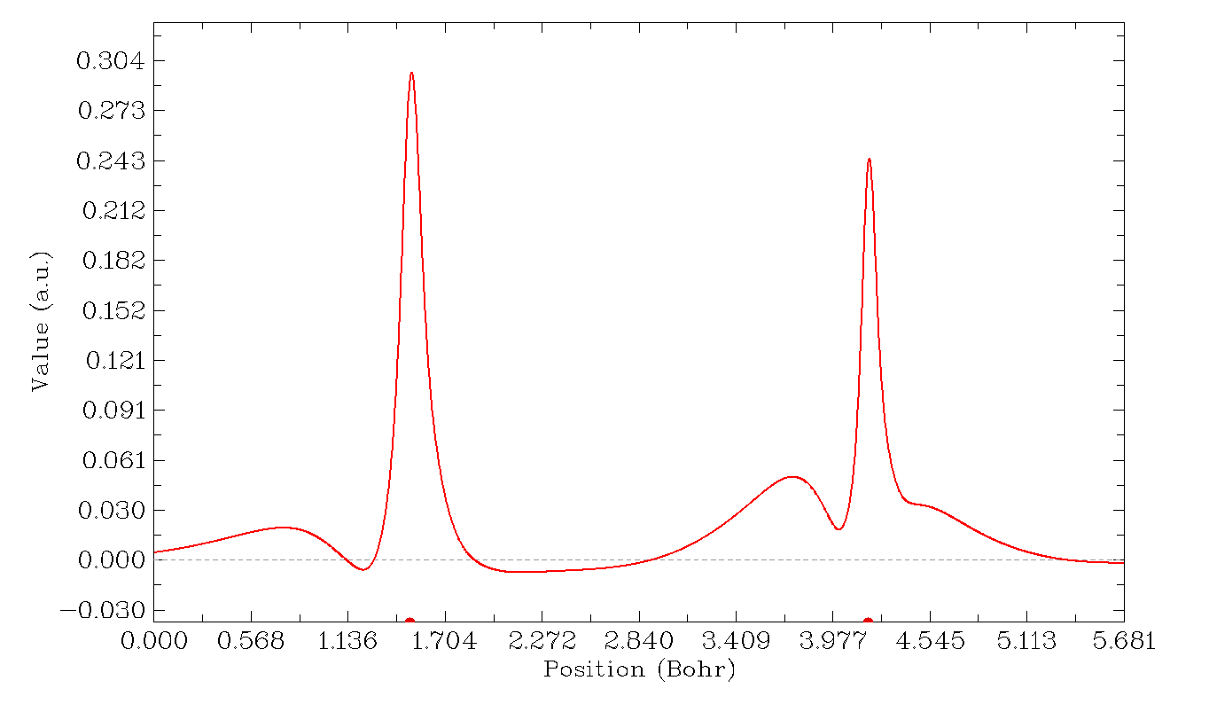
The X-axis corresponds to the position in the line you defined, the dashed line corresponds to the position of Y=0, the left and right red circles denote the position of the first and the second atoms you selected. After clicking right mouse button on the graph to close it, a new menu appears on command-line window, you can save graphic file, adjust the range of Y-axis, export X-Y data points and replot the graph and so on by corresponding options. By selecting option 6, minimum and maximum positions can be located:

Local maximum X:    0.753677  Value:    0.20104903D-01
Local minimum X:    1.219518  Value:   -0.55161276D-02
Local maximum X:    1.503567  Value:    0.29655008D+00
Local minimum X:    2.145518  Value:   -0.70202704D-02
Local maximum X:    3.736194  Value:    0.51047629D-01
Local minimum X:    4.006988  Value:    0.18918295D-01
Local maximum X:    4.184992  Value:    0.24448996D+00
Totally found    3 local minimum,    4 local maximum

Using the same procedure illustrated above, you can plot curve map for any real space function supported by Multiwfn, please have a try.

4.3.2 Study Fermi hole and Coulomb hole of H₂

Note

This is a relatively advanced example, you can skip this section if you are a newbie of quantum chemistry.

In this example we will plot correlation hole (Fermi hole and Coulomb hole) along the axis of H₂. This is an advanced topic, if you are not familiar with the concept of correlation hole, please consult the discussion in part 17 of Section 2.6.

Hartree-Fock wavefunction is capable to exhibit Fermi correlation, but Coulomb correlation is completely omitted. In this case exact Fermi hole can be calculated and plotted by Multiwfn. If Coulomb hole is needed to be analyzed, then post-HF wavefunction must be employed. In current version, Multiwfn is able to evaluate and plot approximate Fermi hole and Coulomb hole for post-HF wavefunctions by Müller approximation, which makes use of natural orbitals to mimic exact pair density. Although the approximation is introduced, the result is generally at least qualitatively correct.

First, we optimize and generate .wfn file for H₂ under CCSD/cc-pVTZ level. CCSD is the highest level of wavefunction that can be generated by Gaussian program (If higher level of wavefunction is needed, you must resort on other programs, see Section 4.A.8 for details). The file has already been provided as examples\H2_CCSD.wfn. The coordinate of H1 is (0.0, 0.0, 0.7016) Bohr, the coordinate of H2 is (0.0, 0.0, -0.7016) Bohr.

Correlation hole involves coordinates of two electrons, to visually study it we must determine position of a reference electron. In this example, we set reference point at (0.0,0.0,-0.3) Bohr. Therefore, we open settings.ini, change refxyz parameter to 0.0,0.0,-0.3.

The correlation hole we first analyzed is Fermi hole (also known as exchange hole), so we change paircorrtype in settings.ini to 1. Since this is closed-shell system, the results for α or β electron are exactly the same, while for open-shell system, you should use "pairfunctype" in settings.ini to select which type of spin electrons will be studied, you can also choose to study exchange-correlation density or correlation factor by adjusting this parameter.

Now boot up Multiwfn, input following commands

examples\H2_CCSD.wfn
3  // Draw curve map
17  // Correlation hole
1  // Defining the line by nuclear coordinate of two atoms
2,1  // Draw curve graph along H2 and H1

Then you will see

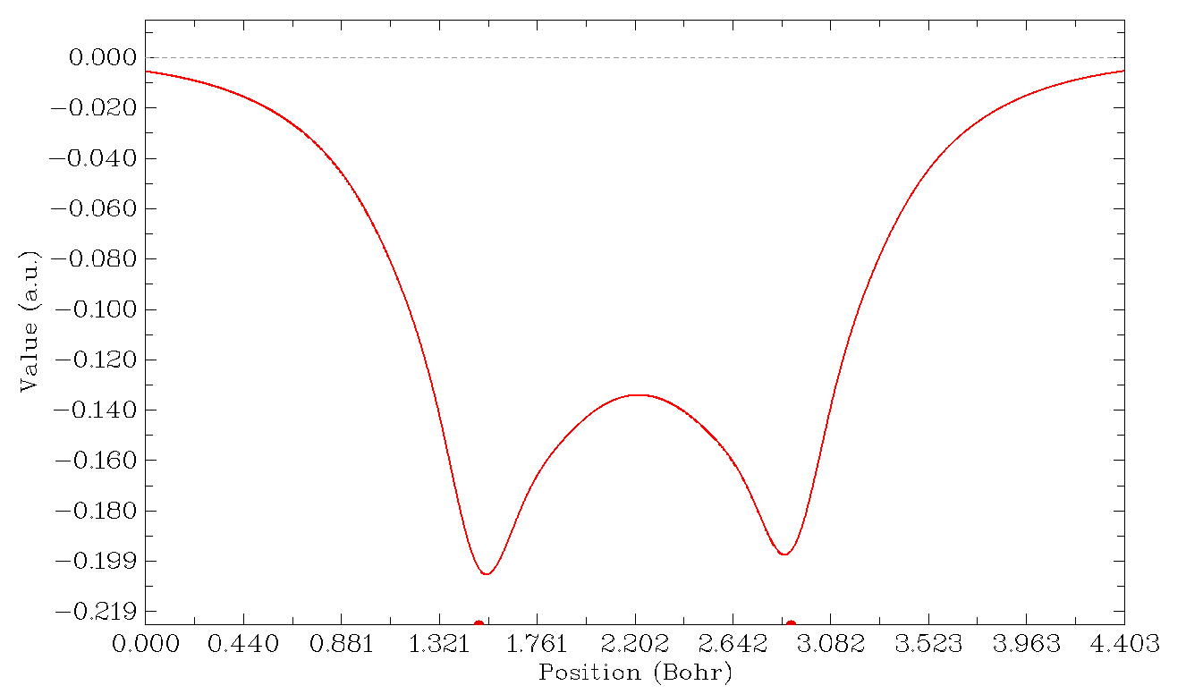
This graph suggests that if we place an α electron at (0.0,0.0,-0.3), then the probability of finding another α electron around the two nuclei will be significantly decreased by almost identical extent due to Pauli repulsion between like-spin electrons. In the H-H bonding region, the probability also obviously decreases. According to Bader's statement "An electron can go where its hole goes and, if the Fermi hole is localized, then so is the electron" (p251 in Atoms in molecules - A quantum theory), we can say that if an α electron presents at (0.0,0.0,-0.3), then it must be able to easily delocalize over the whole H₂ molecular space.

Now we study Coulomb hole. Close Multiwfn, change "paircorrtype" to 2, reboot Multiwfn and then replot the curve graph by using the same procedure, you will see

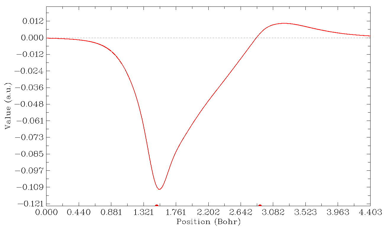
The red dots at left and right sides highlight position of H2 and H1, respectively. How can I infer the position of the reference point on the graph? From the prompt "Set extension distance for mode 1, current: 1.500000 Bohr" we know that the plotting range is extended by 1.5 Bohr in both sides relative to Z coordinates of H2 and H1, and we know that Z coordinate of reference point is larger than H2 by about 0.4016 Bohr, so the reference point on the graph above is 1.5+0.4016=1.9016 Bohr (If you want to highlight the position of reference point on the graph, you can select "4 Draw a vertical line at specific X" and input 1.9016, then redraw the graph via option -1). The graph above reveals that owing to Coulomb repulsion, the probability of finding another electron (α or β) around the hydrogen closest to the reference electron (namely around H2) is largely decreased. As compensation, the probability is increased at backside of H1.

Finally, we study the collective effect of Fermi correlation and Coulomb correlation. Change "paircorrtype" to 3, and plot the line graph again, you will see

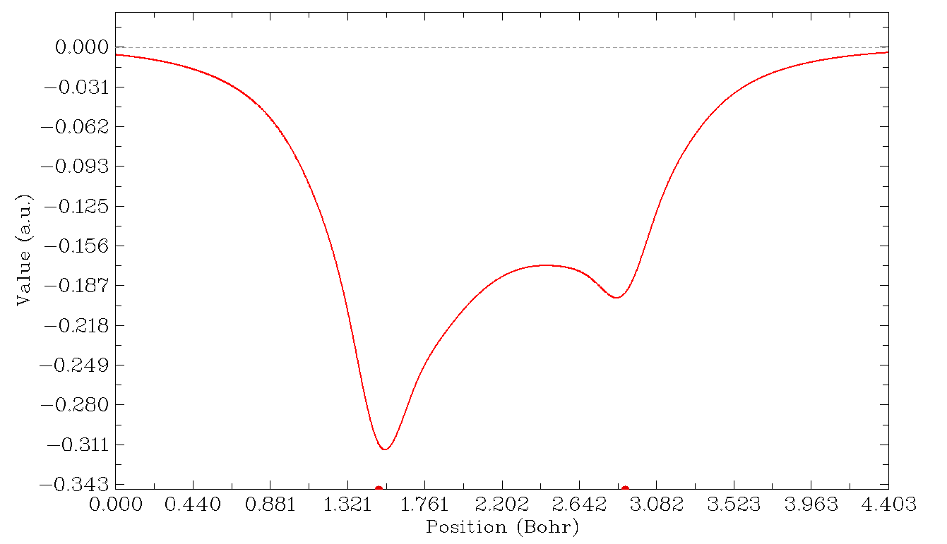
This graph is actually the sum of the first two graphs. From this graph it is clear that the probability decrease of finding an electron (α or β) around the hydrogen closest to reference electron is more severe than that around another hydrogen.

4.3.3 Study interatomic interaction via PAEM-MO method

Note

This is a relatively advanced example, you can skip this section if you are a newbie of quantum chemistry.

In J. Comput. Chem., 35, 965 (2014), the authors proposed a method named PAEM-MO to reveal the nature of interaction between two atoms (covalently or non-covalently bounded). In this example I will briefly introduce this method and show how to realize PAEM-MO analysis in Multiwfn.

PAEM (potential acting on one electron in a molecule) refers to the total potential acting on an electron at point r, and can be written as \(V_{\mathrm{PAEM}}(\mathbf{r})=-V_{\mathrm{ESP}}(\mathbf{r})+V_{\mathrm{XC}}(\mathbf{r})\); where \(V_{\mathrm{ESP}}\) is molecular electrostatic potential and has been introduced in part 12 of Section 2.6. -\(V_{\mathrm{ESP}}\) can be regarded as the classical potential acting on an electron in the system, while the exchange-correlation (XC) potential \(V_{\mathrm{XC}}\) represents the important correction to the classical potential due to quantum effect. \(V_{\mathrm{XC}}\) has two components, namely correlation potential (\(V_{\mathrm{C}}\)) and exchange potential (\(V_{\mathrm{XC}}\)); in fact, only the latter is important, that means even the potential obtained at Hartree-Fock level is in general a good approximation to exact \(V_{\mathrm{XC}}\).

In wavefunction theory, the exchange-correlation potential can be explicitly written as \(V_{\mathrm{XC}}(\mathbf{r})=\frac{1}{\rho(\mathbf{r})}\int\frac{\Gamma_{\mathrm{XC}}(\mathbf{r},\mathbf{r}')}{\left|\mathbf{r}-\mathbf{r}'\right|}\mathrm{d}\mathbf{r}'\), where Γ is known as exchange-correlation density, see part 17 of Section 2.6 for detail. In DFT theory, the XC potential directly comes from the variation of exchange-correlation functional with respect to electron density, i.e. \(V_{\mathrm{XC}}(\mathbf{r})=\delta E_{\mathrm{XC}}[\rho(\mathbf{r})]/\delta\rho(\mathbf{r})\). The \(V_{\mathrm{XC}}\) can be used in Multiwfn in terms of user-defined function. If parameter "iuserfunc" is set to 33, then \(V_{\mathrm{XC}}\) will be calculated based on Γ; if it is set to 34, \(V_{\mathrm{XC}}\) will be evaluated in terms of DFT XC potential, in this case the computational cost is several times lower than 33. For more information, please check corresponding description in Section 2.7.

The essence of HF and KS-DFT theories is the one-electron eigenvalue equation

\[\hat{h}\varphi(\mathbf{r})=\varepsilon\varphi(\mathbf{r})\]

where

\[\hat{h}=-(1/2)\nabla^2+V_{\mathrm{PAEM}}(\mathbf{r})\]

Solving the equation results in a set of MOs {\(\varphi\)}, their eigenvalues correspond to the energy of the electrons running in the orbitals.

According to the viewpoint of PAEM-MO, if the energy of an occupied MO is higher than the barrier of \(V_{\mathrm{PAEM}}\) between a pair of atoms, then the electrons in this MO will be able to freely delocalize over the two atoms, and thus have direct contribution to covalent bonding.

Below I present two very simple examples of using PAEM-MO method to judge the type of interatomic interaction. More examples and discussions can be found in J. Comput. Chem., 35, 965 (2014).

H-H interaction in hydrogen molecule

First set "iuserfunc" in settings.ini to 33, then user-defined function will be equivalent to the \(V_{\mathrm{XC}}\) evaluated based on Γ. Boot up Multiwfn and input below commands

examples\H2.fch  // Produced at HF/def2-TZVP level
3  // Plot real space function along a line
100  // User-defined function
0  // Adjust extension size at both sides
3  // 3 Bohr, which is larger than the default value
1  // Use two nuclei to define the line
1,2

Close the graph, then adjust some plotting parameters to make the graph better

11  // Change length unit of the graph to Å
3  // Change range of Y axis
-3,0.1  // From -3.0 a.u. to 0.1 a.u.
10  // Set label intervals of X and Y axes
0.5,0.5
-1  // Replot

You will see the graph below, which exhibits the PAEM curve along the H₂ axis

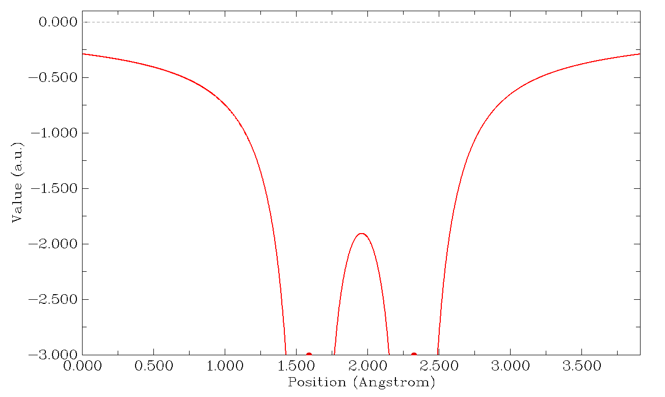
As you can see, there is a barrier of PAEM around the midpoint of H-H bond. In order to locate the exact value of the barrier, we close the graph and select 6. From the output we find the maximum of the curve is -1.903 a.u. (-51.78 eV). Present system only has one doubly occupied MOs, whose energy (-16.23eV) significantly exceeded the PAEM barrier, implying that the electron is not confined in any hydrogen atom but substantially contributes to the H-H binding, so the H-H bond must be covalent.

He-He interaction in He₂

Please plot PAEM curve along the He-He axis in He₂ with the same steps as above. The wavefunction file used here is examples\He2.fch, which was produced at HF/def2-TZVP level at separation of 2.97 Å (a reasonable distance). The resultant graph should look like below

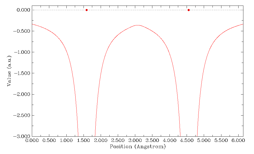
Obviously, the PAEM barrier (-9.78 eV) is higher than that in the case of H₂. The energy of the two doubly occupied MOs are -25.03 and -24.91 eV respectively, both of them are lower than the barrier, therefore the electrons in each He atom are difficult (but not completely impossible due to tunnel effect) to overcome the barrier to freely delocalize to another He. The He-He interaction thus should be regarded as noncovalent interaction.

Note that in the original paper of PAEM-MO the PAEM is evaluated based on the expensive CISD wavefunction, while we merely use HF wavefunction. However, our results are in good agreement with that at CISD level, showing that correlation potential may be safely neglected in the study of PAEM.

The interested users are suggested to replot the PAEM with iuserfunc=34 to employ DFT XC potential in PAEM, you will find the results are very similar to those we obtained earlier.

It is noteworthy that, although the PAEM-MO analysis method has clear physical meaning, its many limitations severely hinder it to be a universal method to distinguish covalent and noncovalent interactions like ELF or LOL: (1) PAEM-MO analysis does not always present reasonable conclusion in all cases. For example, PAEM-MO erroneously indicates that the H-bond in water dimer is covalent interaction. (2) PAEM-MO is difficult to apply to polyatomic molecules, since there are often too many occupied orbitals with complex shapes. (3) If the two atoms are placed too close to each other, then PAEM-MO almost always indicates that the interaction is covalent.