4.0 View orbitals and structure

In this section, I will first introduce how to use the built-in interface for visualizing various kinds of orbitals, then in Section 4.0.3, I will show how to use Multiwfn in combination with VMD to easily and quickly plot state-of-art orbital graphs.

4.0.1 Viewing molecular orbitals of cycloheptatriene

Boot up Multiwfn, input examples\cycloheptatriene.fch and press ENTER button, then select main function 0, a GUI window will pop up, meanwhile information of all atom coordinates along with basic information of featured molecular orbitals are printed on Multiwfn console window.

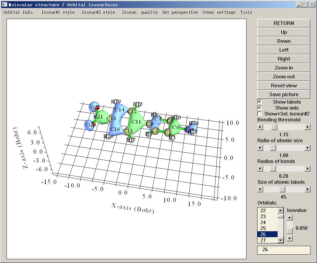
You can zoom in/out the system by scrolling mouse wheel, and rotating the system by clicking Up/Down/Left/Right buttons on the right side of the GUI. You can also freely rotate the system by dragging it in the drawing region via left mouse button; you can also hold the Ctrl key and drag the system with left mouse button horizontally and vertically to rotate it along the screen and zoom in/out, respectively; moreover, you can hold down the Shift key and drag the system to translate it. Note that if you are using Linux version, the aforementioned mouse dragging operations will be available only after clicking the drawing region once to make the icon become a hand.

You can also adjust bonding threshold, adjust size of atom spheres and labels, save the graph as image file, and so on, via corresponding widgets on the right side of the GUI. See Section 3.2 for more information.

The numbers in the right-bottom list are orbital indices, you can view orbital isosurface by selecting corresponding index, or directly inputting the orbital index in the text box and then press ENTER button. Note that if your system is unrestricted open-shell, to select beta orbital you should input negative index, for example, -5 corresponds to the 5th beta orbital. Plot two orbitals simultaneously in this window is also possible, as illustrated in Section 4.0.2.

For convenience, if your input file records R/U/RO(HF/KS) wavefunction, you can directly input orbital label in the text box at right-bottom corner. For example, inputting h stands for choosing HOMO, l+2 corresponds to LUMO+2, la corresponds to LUMO of alpha, hb-3 corresponds to HOMO-3 of beta, etc.

The green and blue isosurfaces correspond to positive and negative parts, respectively. The isovalue can be adjusted by dragging slide bar, you can also input its value via “Set isovalue” option in “Other settings” drop-down list at the top of the GUI. Isosurface style and colors and be altered by corresponding suboptions in "Isosur#1 style". The quality of the isosurface can be set by the options in "Isosur. quality".

By selecting "Orbital info."-"Show all", energy, occupation number and type of all orbitals will be shown in Multiwfn console window. If you do not want too many high-lying virtual MOs to be shown, you can choose "Show up to LUMO+10" or "Show occupied orbitals". If irreducible representations are recorded in the loaded .mwfn/molden/gms file, then they will be shown as the last column.

In the "Other settings" and "Tools" of the menu bar, there are many useful options, please play with them, and when you are confused, see Section 3.2 for explanation. The "Tools” - “Batch plotting orbitals" is quite worth noting, via this tool you can very conveniently save a lot of selected orbitals to respective image file in current folder, see https://youtu.be/SHwrQhqBHZ0 for video illustration.

If you want to plot probability density of an orbital instead of its wavefunction, you can choose “Other settings” - “Choose plotting wavefunction or density”, and then choose “Density”.

To close the window, click “RETURN” button. More detailed explanation about this interface can be found in Section 3.2.

Note

Visualizing isosurface of Rydberg orbitals by main function 0 of Multiwfn is also possible, however, since they show very diffuse character, in order to avoid truncating of isosurfaces, you should select "Other settings"-"Set extension distance" in the menu, and then input a relatively large value, for example, 12 (the unit is Bohr), then select the orbital to visualize it. The default value of extension distance is controlled by "Aug3D" in settings.ini. An example of visualizing Rydberg orbitals is given in Part 2 of Section 4.200.5.

Tip: Recommendation of the steps for obtaining pretty orbital isosurface graph

• Enter main function 0, select the orbital to be visualized, properly set isovalue

• Click "Show Labels" to disable axis

• Properly adjust viewpoint

• Properly change the size of atomic labels. Note that type of labels can be changed via "Set atomic label type" in "Other settings" at menu bar

• If the rendering effect of the isosurface is not quite good, use "Set lighting" in "Other settings" to adjust lighting.

• Select "Isosur. quality" in the menu bar, set to "high-quality" (medium sized system) or "very high-quality" (large system).

• Click "Save picture". Use such as Irfanview or Photoshop program to open it, shrink the size of the image file to 50% (in this process resample will be automatically done, making anti-aliasing effect effectively realized), then properly crop the graph.

  Here is an example obtained via above steps, the quality is pretty good

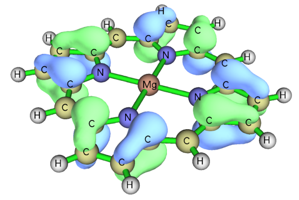
It is suggested to use "face+mesh" drawing style instead of the default "solid face", since in this case the saved picture will be more stereoscopic.

4.0.2 Viewing natural bond orbitals (NBO) of ethanol

There are two ways to view NBOs, if you are a Gaussian user, way 2 may be more convenient, however if you also need to view natural hybrid orbital (NHO) or natural atomic orbital (NAO) or some other types of orbitals generated by NBO program, you have to use way 1.

Way 1: Using NBO plot files

The common way is to generate NBO plot files (.31~.40) and load them into Multiwfn. To generate these files by Gaussian, you should add pop=nboread in route section, that means the keywords of NBO at the end of input file will be passed to NBO module (Link 607 in Gaussian), then add for example $NBO plot file=C:\NH2COH $END at the end of the input file with a blank line before it, you can refer to the NH2COH_NBO.gjf in “example” directory. Run the input file by Gaussian, you will find that NH2COH.31, NH2COH.32 ... NH2COH.41 have been generated in C: folder. The NH2COH.31 and NH2COH.37 have already been provided in “example” folder. Now boot up Multiwfn and input following commands

examples\NH2COH.31  // .31 file contains necessary basis function information for plotting
examples\NH2COH.37  // .37 file contains NBO information. .32~.40 files correspond to PNAO/NAO/PNHO/NHO/PNBO/NBO/PNLMO/NLMO/MO respectively. Hint: You can only input 37, because in present example the .37 and the .31 file share the same name
0  // Enter the GUI

You can choose corresponding NBO orbital from right-bottom list to view the isosurface. Multiwfn is also capable to plot two orbitals simultaneously, for instance, here we will plot NBO 12 and NBO 56, which correspond to occupied lone pair of nitrogen atom and unoccupied anti-π bond between carbon and oxygen atoms respectively. Firstly, we choose 12 from the orbital list to plot NBO 12, and then click "Show+Sel. isosur#2", after that we click 56 in the list, you will see both of NBO 12 and NBO 56 are shown. The yellow-green and purple parts of NBO 56 (isosurface#2) correspond to positive and negative parts, respectively.

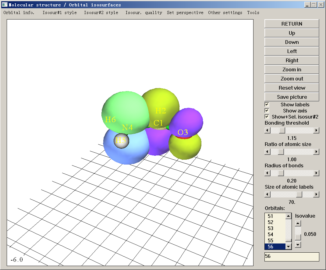
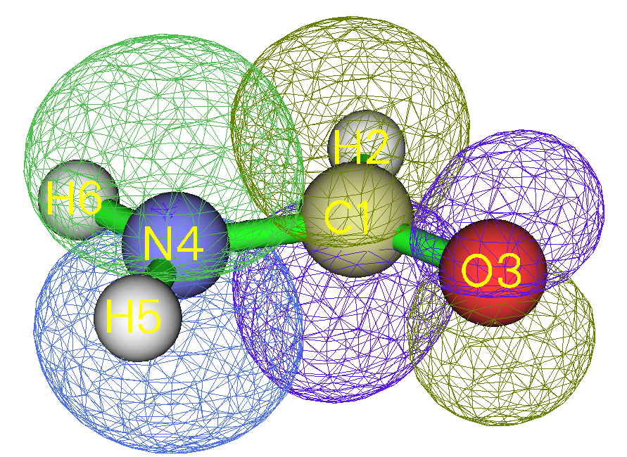
It is somewhat difficult to study overlapping extent between the two orbitals from the solid face graph, so we choose "Use mesh" in "Isosur#1 style" and the counterpart in "Isosur#2 style" to make the two isosurfaces represented as mesh, see below. (Please also try "transparent face" style) Now the overlapping extent become distinct, it is quite clear that NBO 12 substantially overlapped with NBO 56, the resulting strong delocalization is one of the main reasons why the second-order perturbation energy between them is very large (~60 kcal/mol). In Section 4.4.5, you will learn how to obtain a contour map for the two orbitals.

Note

Notice that for unrestricted calculations, .32 and .33 files outputted by NBO 3.1 module in Gaussian are incorrect -- the title parts are missing, which will lead to strange result, you should fix them by consulting other plot files such as .34, it is very easy.

Regarding the ways to pass the keywords for generating NBO plot files to NBO module in other quantum chemistry packages, please consult corresponding manual. You can also use stand-alone version of NBO program (GENNBO) to generate NBO plot files, an input file (.47) needs to be prepared first. To generate it, you should load a file containing basis function information into Multiwfn, then enter main function 100, select subfunction 2, then choose corresponding option to export .47 file. After that, manually add plot keyword between “$NBO” and “$END” in the .47 file. Then if you use GENNBO program to run the .47 file, you will get NBO plot files.

Way 2: Using .fch file as NBO information carrier

Gaussian provides a keyword pop=saveNBO, if you add it in your Gaussian input file, NBOs will be saved to checkpoint file instead of MOs. You can use corresponding .fch file as Multiwfn input file to view NBOs. If theoretical level of the task is HF or DFT, you should add saveNBOene in the first line of the .fch file; if post-HF method is used and density keyword has also been specified, you should add saveNBOocc in the first line of the .fch file, in this case Multiwfn will do some special treatments internally. However, if your aim is just viewing NBOs in main function 0, you can ignore this step.

Beware that when Gaussian storing the NBOs to checkpoint file, they may be automatically reordered. For example, you may see the information like below in the Gaussian output file:

Reordering of NBOs for storage:     7    8    3    1    2    4    6    5    9   38 ...

That means the 1st, 2nd, 3rd, 4th ... orbitals in the .chk/.fch file in fact correspond to the 7th, 8th, 3rd, 1st ... NBOs generated by the NBO module, respectively.

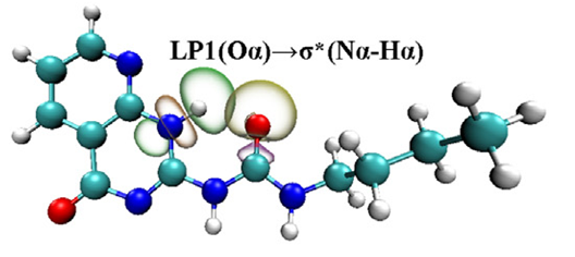
It is worth to note that if you use Multiwfn in combination with VMD, you can plot very pretty NBO isosurface maps, see my blog article "Using Multiwfn to plot NBO and related orbitals" (in Chinese, http://sobereva.com/134) for detail. Here is a map plotted by a Multiwfn user in his work J. Mol. Graph. Model., 59, 31 (2015).

4.0.3 Using Multiwfn + VMD to rapidly plot high-quality orbital isosurface map

Note

Chinese version of this tutorial is my blog articles “Using Multiwfn+VMD to rapidly plot high-quality isosurface map of molecular orbitals” (http://sobereva.com/447) and “Method of drawing state-of-the-art orbital isosurface map using VMD in combination with Multiwfn” (http://sobereva.com/449).

Video illustration corresponding to this section is available at https://youtu.be/-3TXfdO8H7s, please never forget to look at it!!!

Prologue

If one employs Multiwfn to export cube file for the orbitals of interest, and then render them as isosurface map in VMD (http://www.ks.uiuc.edu/Research/vmd/), very ideal orbital isosurface map can be obtained, the procedure has been detailedly described in my blog article "Using Multiwfn to visualize molecular orbitals" (in Chinese, http://sobereva.com/269). However, the procedure introduced in this article is somewhat lengthy, many manual operations are needed. In order to simplify the procedure as much as possible, here I show how to use scripts to very easily and quickly draw high-quality orbital isosurface map by using Multiwfn and VMD in combination. In this section I only illustrate how to plot MOs, but the same procedure can also be applied for plotting other kinds of orbitals, however you need to properly modify the input stream file (see below). If you do not know how to run Multiwfn in silent mode, I suggest you read Section 5.2 first so that you can better understand this section. Here I assume you are using Windows system, for Linux platform you should manually write corresponding script. The VMD program I used here is version 1.9.3.

Preparation work

Copying showorb.bat and showorb.txt from "examples\scripts" to the folder containing Multiwfn executable file.

The showorb.bat is a Windows batch process file, it is used to invoke Multiwfn to calculate grid data of wavefunction for selected orbitals and then move the exported cube files to VMD folder. You should manually edit this file to make the input file path correspond to the actual path of input file, and then replace the VMD folder in this file with actual VMD folder in your machine.

The showorb.txt is input stream file, each line corresponds a command needed to be inputted in the Multiwfn interactive interface. You should manually set the third line as indices of the orbitals you want to plot, for example, 10,20-23,28-30.

The showorb.vmd in "examples\scripts" is a VMD plotting script, you should copy it to VMD folder, and then add source showorb.vmd to the end of the vmd.rc file in VMD folder, so that the script will be automatically executed when VMD boots up. This script defines three customized commands:

• orb i: Used to load cube file of orbital i and show it as isosurfaces. The default isovalue is 0.05, you can change it by editing showorb.vmd

• orbiso x: Used to change the isovalue to x.

• orbclean: Used to delete all orbital cube files in VMD folder.

Example

Here we plot MOs for examples\excit\D-pi-A.fchk. Make sure that all preparation works have done, then edit the showorb.bat, replace the default input file 1.fch with examples\excit\D-pi-A.fchk, and ensure that the actual VMD folder has been properly specified in this file. Then open showorb.txt, set the third line as 54-59, so that we can visualize MOs from 54 to 59. Then double-click the showorb.bat, Multiwfn will be invoked to load input file, calculate and export grid data of wavefunction for the selected orbital. For e.g. orbital 54, the exported file will be named orb000054.cub. All the orbital cube files are then automatically moved to the VMD folder. After that, boot up VMD, input orb 56 in VMD console window, then orb000056.cub will be loaded into VMD and drawn as isosurfaces:

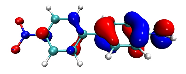
In the map above, positive and negative phases are represented as red and blue colors, respectively. "Glossy" material is used by default. If you want to change the color or material, you should enter "Graphics" - "Representation" and modify corresponding options. You can also change default color and material by modifying the showorb.vmd script.

If then you want to visualize another orbital, for example MO54, then simply input orb 54 in the VMD console window.

If you want to change the isovalue to e.g. 0.02, simply input orbiso 0.02.

If after visualization, you want to clean all orbital cube files in the VMD folder, just input orbclean, then all orb??????.cub files will be deleted.

By default, "medium-quality grid" (about 512000 points) is used to calculate orbital wavefunction, this is adequate for small and medium sized systems. However, for large systems, such as those consisting of one hundred atoms or more, you must employ higher number of grid points. If you want to change the default grid to "high-quality grid", you should set the fourth line in showorb.txt to 3. In addition, as mentioned in Section 4.0.1, for visualizing Rydberg orbitals you must increase extension distance of grid data. To do so, you should add

-10
12

between the third and fourth lines of showorb.txt, then extension distance will be increased from default value to 12 Bohr.

Plot state-of-the-art orbital isosurface map

If you want to obtain an even better orbital isosurface graph, just follow below procedure (please use VMD 1.9.3, DO NOT use other VMD version!):

• (1) Plot an orbital in VMD as described above

• (2) Copy all content in examples\scripts\VMDrender.txt to VMD console window to modify the plotting setting

• (3) In VMD, select "File" - "Render" - "Tachyon", click "Start Rendering". Then vmdscene.dat will appear in VMD folder, it is input file of the Tachyon render.

• (4) Copy the examples\scripts\VMDrender_full.bat to VMD folder

• (5) Double click the VMDrender_full.bat, then the Tachyon render (tachyon_WIN32.exe) in VMD folder will be invoked to carry out render. After a while, full.bmp appears in the VMD folder, it is the produced image file.

The rendered image of MO56 of examples\excit\D-pi-A.fchk is shown below, the graph looks extremely good!

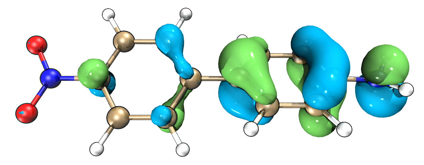
The rendering time is fairly long for large systems. For saving time, you can use the VMDrender_noshadow.bat instead of the VMDrender_full.bat, in this case no shadow effect will be observed in the resulting graph, while the rendering cost is correspondingly reduced.

Sometimes, especially for large systems, the shadows cast by the transparent orbital isosurfaces make the graph look too dark, you can manually add -shadow_filter_off argument in the .bat file to disable this kind of shadow during rendering.