4.200 Other functions (Part 2)
4.200.5 Plot radial distribution function of electron density
Multiwfn is capable of plotting radial distribution function (RDF) for any real space function, see Section 3.200.5 for detail. This function is particularly useful for studying electronic structure character of sphere-like systems.
This section consists of two parts. In part 1, we will plot RDF for electron density of fullerene (C60); while in part 2, I will show how to plot RDF of electron density for a Rydberg orbital to characterize it quantitatively.
Part 1: RDF of electron density for fullerene
Since .wfn file of fullerene at B3LYP/6-31G* level is large, I only provide the corresponding Gaussian input file for you (C60.gjf in "example" folder), please properly modify and run it by Gaussian to produce C60.wfn.
Boot up Multiwfn and input:
C60.wfn
200 // Other functions (Part 2)
5 // Plot RDF for a real space function
3
1,6 // Set the lower and upper limit of RDF to 1.0 and 6.0 Å, respectively
0 // Calculate RDF and its integration curve
After the calculation is finished, select option 0, below RDF map will be shown on the screen, the X-axis corresponds to radial distance
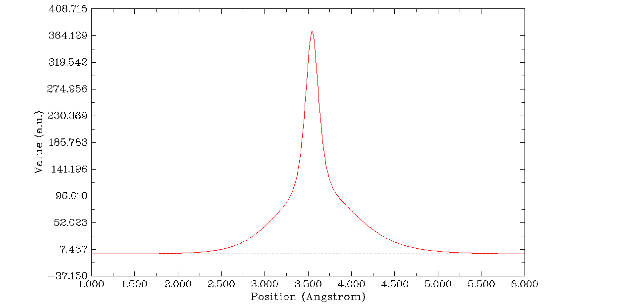
As you can see, the peak of RDF is about 3.5 Å, this is because the distance between nucleus of carbons and the sphere center is 3.545 Å. It is known that electron density has maximum at nuclear position for any atom except for hydrogen.
If you carefully examine the RDF curve, you will find that the curve on the right side of the peak is slightly higher than that on the left sight. The reason is that the amount of π electrons at outer side of fullerene is richer than inner side. You can also draw and analyze ELF isosurface map to confirm this point.
You can also choose option 2 to plot integration curve of RDF, as shown below
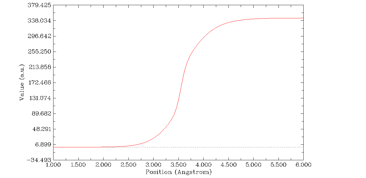
Probably you have noticed that after the calculation there is a prompt on screen:
which means integrating the RDF from r=1.0 to r=6.0 Å yields 344.932, it also corresponds to the value of integration curve at r=6.0. This value deviates evidently from our expectation, namely the number of electrons in current system (360). One reason is that the default number of integration points is not large enough (500 and 2030 for radial and angular parts, respectively. You can manually increase them), while another reason is more important, that is the size of the current system is too large, using single-center integration method is too difficult to yield a very accurate result, at least for integrating electron density.
Part 2: Using RDF of electron density to quantitatively characterize Rydberg orbital for acetone
Rydberg orbitals denote the spatially very diffuse MOs, their orbital shapes are akin to atomic orbitals, since electrons in Rydberg orbitals can be regarded as weakly bounded by a small cation core, which behaves as an atomic nucleus. In order to faithfully represent the diffuse character of Rydberg orbitals, basis set with substantial diffuse functions must be employed, e.g. aug-cc-pVTZ.
The example file we used below is formaldehyde calculated at B3LYP/aug-cc-pVTZ level by Gaussian. We will first visualize Rydberg orbitals as isosurfaces, and then calculate RDF of electron density corresponding to these orbitals to characterize them quantitatively.
Boot up Multiwfn, load examples\H2CO_aVTZ.fch, then enter main function 0. Since Rydberg orbitals are very diffuse, in order to avoid truncating their isosurfaces when viewing them, you should first select "Other settings"-"Set extension distance" and input a large value, here we input 12. After that, change isovalue to a much smaller value than default, e.g. 0.01. Then we arbitrarily select some virtual MOs to examine their features. You will find a lot of virtual MOs show very diffuse character, for example, MO10 and MO11 are shown below:
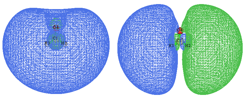
The main distribution region of both of them are far from the molecule. MO10 is almost spherically symmetric, thus can be denoted as s type of Rydberg orbital. While MO11 has two phases, they equally distribute at the two sides, the overall shape is very close to atomic p orbitals, therefore MO11 can be identified as p type of Rydberg orbital.
How to quantitatively demonstrate that the main distribution region of these Rydberg orbitals is far from the molecular center? One of the best ways is plotting RDF of electron density corresponding to these orbitals. Here we plot this kind of RDF map for MO11. We close the GUI of main function 0, and then input below commands:
6 // Modify wavefunction
26 // Modify orbital occupation number
0 // Select all orbitals
0 // Select occupation number of all orbitals to zero
11 // Select orbital 11
2 // Set occupation number of orbital 11 to 2.0 (assume it is doubly occupied)
q // Return
-1 // Return to main menu
200
5 // Plot RDF
3 // Set lower and upper limit of radial plotting
0,10 // From 0 to 10 Å
4 // Set angular number of integration points. The default value is unnecessarily high for present purpose, therefore we set it to a smaller value to reduce computational time
302 // 302 angular points
0 // Calculate RDF for electron density (which is the default real space function)
1 // Plot the RDF map
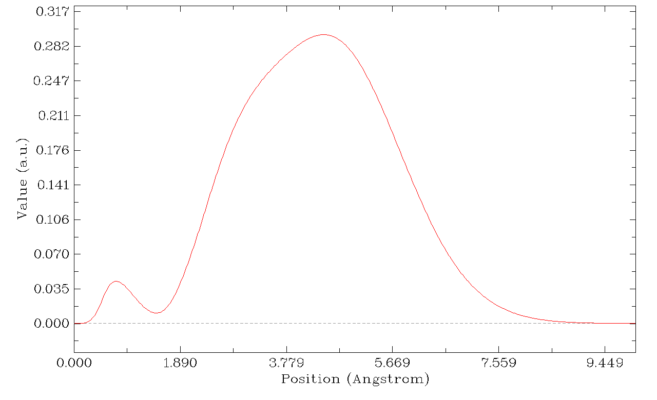
From the map it can be seen that the global maximum peak is at about 4.6Å, indicating that the major distribution region of this orbital wavefunction is very far from origin (in present .fch file, Cartesian origin corresponds to molecular center), and thus MO11 can be unambiguously identified as a Rydberg orbital.
Please also plot such an RDF map for a regular valence virtual MO, e.g. MO9, which is π* orbital. Where is its peak position?
4.200.6 Studying correspondence between orbitals in different wavefunction files
In this section, two examples are given to illustrate how to use the function introduced in Section 3.200.6, this function aims to reveal relationship between orbitals in different wavefunction files.
4.200.6.1 Revealing relationship between HF and MP2 orbitals of CH3NH2
In this section, we study the correspondence between HF/6-31+G* MOs and MP2/6-31+G* natural orbitals (NO) for CH3NH2.
After booting up Multiwfn we input
C:\CH3NH2_MP2.wfn // MP2/6-31+G* wavefunction file, there are 48 NOs
200 // Other function, part 2
6 // Analyze correspondence between orbitals in two wavefunctions
[Press ENTER button directly to choose all orbitals]
C:\CH3NH2_HF.wfn // HF/6-31+G* wavefunction file, there are 9 MOs
[Press ENTER button directly to choose all orbitals]
Then you will see
   1:       2( 94.63%)    1(  5.36%)    4(  0.01%)    3(  0.00%)    6(  0.00%)
   2:       1( 94.64%)    2(  5.36%)    3(  0.00%)    9(  0.00%)    6(  0.00%)
   3:       3( 85.21%)    4(  9.87%)    7(  3.24%)    9(  0.88%)    6(  0.79%)
   4:       4( 86.88%)    3( 10.66%)    6(  1.94%)    9(  0.48%)    7(  0.02%)
   5:       6( 54.88%)    7( 41.11%)    9(  3.20%)    4(  0.45%)    3(  0.34%)
   6:       8( 57.50%)    5( 42.47%)    7(  0.00%)    6(  0.00%)    4(  0.00%)
   7:       5( 57.50%)    8( 42.48%)    7(  0.00%)    4(  0.00%)    6(  0.00%)
   8:       9( 86.62%)    6( 10.30%)    7(  1.63%)    4(  0.89%)    3(  0.50%)
   9:       7( 53.98%)    6( 32.07%)    9(  8.76%)    3(  3.28%)    4(  1.89%)
  10:       9(  0.00%)    7(  0.00%)    6(  0.00%)    4(  0.00%)    2(  0.00%)
  11:       5(  0.00%)    8(  0.00%)    3(  0.00%)    7(  0.00%)    4(  0.00%)
... (ignored)
  47:       6(  0.01%)    7(  0.00%)    9(  0.00%)    3(  0.00%)    4(  0.00%)
  48:       9(  0.04%)    7(  0.00%)    6(  0.00%)    4(  0.00%)    3(  0.00%)
The first column denotes the index of the MP2 NOs, the largest five contributions from the Hartree-Fock MOs to them are shown at right side. As can be seen, the first (second) NO is nearly equivalent to the second (first) MO. While the 9th NO cannot be solely represented by any MO, it mainly arises from the severe mix of the 7th (53.98%) and 6th MOs (32.07%), the 9th MO also has nonnegligible contribution (8.76%).
If you want to get all coefficients and compositions of an orbital of present wavefunction (e.g. the 5th NO), then simply input 5, you will see
    1   Contribution:     0.000 %    Coefficient:    0.001509
    2   Contribution:     0.000 %    Coefficient:   -0.000042
    3   Contribution:     0.339 %    Coefficient:   -0.058201
    4   Contribution:     0.447 %    Coefficient:    0.066869
    5   Contribution:     0.000 %    Coefficient:    0.000000
    6   Contribution:    54.882 %    Coefficient:    0.740826
    7   Contribution:    41.113 %    Coefficient:   -0.641194
    8   Contribution:     0.000 %    Coefficient:    0.000000
    9   Contribution:     3.199 %    Coefficient:   -0.178856
Total:    99.980 %
this output shows that \(\displaystyle |\mathrm{NO}\ 5\rangle=0.7408\,|\mathrm{MO}\ 6\rangle-0.6412\,|\mathrm{MO}\ 7\rangle-0.1788\,|\mathrm{MO}\ 9\rangle\cdots\) The 99.98% at the last line indicates that the 5th NO can be perfectly represented by linear combination of these nine MOs.
4.200.6.2 Study contribution of lone pair of nitrogen to MOs of dopamine
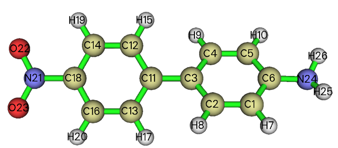
Sometimes it is useful to investigate a problem like "How large is contribution of lone pair of a heteroatom to a molecular orbital?", using orbital localization technique in combination with subfunction 6 of main function 200 can provide a clear answer to this problem. In this section, we will study contribution of lone pair of nitrogen in amino group to occupied MOs for a Donor-π-acceptor type of molecule. The wavefunction file is examples\excit\D-pi-A.fchk, the structure and atomic numbering are shown below
We should first generate localized molecular orbitals (LMOs), because commonly a lone pair can be represented by an LMO.
Boot up Multiwfn and input below commands
examples\excit\D-pi-A.fchk
19 // Orbital localization analysis
1 // Localize occupied orbitals
The LMOs are automatically exported to new.fch in current folder. From the outputted LMO composition on the screen, we can find there are several LMOs closely related to the N24, namely the nitrogen in amino group. Below are relevant lines of orbital composition output.
    4:  24(N ) 99.3%        5:  18(C ) 98.9%        6:   6(C ) 98.6%
...
   19:  24(N ) 60.1%  25(H ) 32.9%        20:  21(N ) 57.5%  18(C ) 33.7%
   27:   2(C ) 45.6%   3(C ) 44.5%        28:  24(N ) 53.6%   6(C ) 37.8%
   33:  23(O ) 65.8%  21(N ) 27.5%        34:  24(N ) 59.9%  26(H ) 33.2%
   43:   5(C ) 46.2%   4(C ) 44.9%        44:  24(N ) 77.7%   6(C )  9.9%
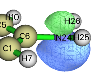
To confirm which one corresponds to lone pair of N24, we enter main function 0 and check isosurface of the highlighted LMOs one by one, we find LMO 44 can be regarded as lone pair orbital of N24, the isosurface map with isovalue of 0.1 is shown below
Now we can check contribution of this LMO to various MOs. Reboot Multiwfn and input
examples\excit\D-pi-A.fchk
200 // Other functions (Part 2)
6 // Analyze correspondence between orbitals in two wavefunctions
1,56 // We want to check all occupied MOs (indices range is 1~56)
new.fch // The file containing LMOs
44,44 // Only the 44th orbital in the new.fch will be taken into account
From the output, we can find some MOs have large composition of the LMO 44, relevant lines are shown below (Since only LMO 44 is taken into account, other LMOs have exactly zero contribution)
    44:     44( 10.04%)   43(  0.00%)   42(  0.00%)   41(  0.00%)   40(  0.00%)
*   45:     44(  8.73%)   43(  0.00%)   42(  0.00%)   41(  0.00%)   40(  0.00%)
*   49:     44( 33.29%)   43(  0.00%)   42(  0.00%)   41(  0.00%)   40(  0.00%)
*   53:     44( 14.28%)   43(  0.00%)   42(  0.00%)   41(  0.00%)   40(  0.00%)
*   56:     44( 19.74%)   43(  0.00%)   42(  0.00%)   41(  0.00%)   40(  0.00%)
We return to main menu, enter main function 0 and visualize MO 49 to check whether LMO 44 (lone pair of N24) really has large contribution (33.29%) to it. The isosurface map with isovalue of 0.05 is shown below
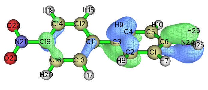
As can be seen, indeed MO 44 is largely contributed by lone pair of N24, since a large part of its isosurface covers the lone pair region of N24, the computed composition 33.29% should be a reasonable value.
4.200.12 Calculate energy index (EI) and bond polarity index (BPI)
In this section I will illustrate how to calculate EI and BPI indices, which were defined in J. Phys. Chem., 94, 5602 (1990). If you are not familiar with these two quantities, please read Section 3.200.12 first. The geometry and wavefunction involved in this example were produced at HF/6-31G* level, which is the one used in above-mentioned paper.
We will calculate BPI for C-N bond of CH3NH2, before this we first need to calculate reference EI value for C and N atoms, which correspond to EI of C in ethane and N in H2N-NH2, respectively. Boot up Multiwfn and input
examples\EI_BPI\ethane.fch
200 // Other function, part 2
12 // Calculate energy index (EI) or bond polarity index (BPI)
1 // C1 atom
You will see the EI value for C in reference molecule ethane is -0.667639 a.u.
Reboot Multiwfn and input
examples\EI_BPI\N2H4.fch
200 // Other function, part 2
12 // Calculate EI or BPI
1 // N1 atom
You can see the EI value for N in reference molecule H2N-NH2 is -0.718126 a.u.
Next we calculate EI for C and N in CH3NH2. Reboot Multiwfn and input
examples\EI_BPI\CH3NH2.fch
200 // Other function, part 2
12 // Calculate EI or BPI
1 // C1, the result is -0.693374 a.u.
5 // N5, the result is -0.698092 a.u.
The BPICN in CH3NH2.is computed as
As a comparison, use examples\EI_BPI\F2.fch to calculate reference value for F, the result should be -0.992542 a.u., and use examples\EI_BPI\CH3F.fch to calculate EI for C and F in CH3F molecule, the result should be -0.750302 and -0.885961, respectively. Then compute the BPICF value as -0.750302+0.667639+0.885961-0.992542= -0.189. Since BPICF in CH3F is evidently more negative than BPICN in CH3NH2, it can be concluded that C-F bond in CH3F is more polar than C-N bond in CH3NH2.
Via EI index we can also evaluate the so-called group electronegativity, which is often more useful than atomic electronegativity. Here we calculate electronegativity for -CH3 group, which is simply the negative of EIC for CH3 radical. Boot up Multiwfn and input
examples\EI_BPI\CH3.fch // Optimized and produced at UHF/6-31G*
200 // Other function, part 2
12 // Calculate EI or BPI
1 // Carbon atom
The result is -0.630656 a.u., corresponding to electronegativity of CH3 group of 0.631. Then we use examples\EI_BPI\F.fch to calculate group electronegativity for -F, the result is 0.957. It is clear that -F group has much higher electronegativity, and thus has stronger capacity to attract electrons than -CH3 group due to its lower average energy per valence electron.
4.200.13 Study orbital contributions to density difference
Note
Chinese version of this section is my blog article “Using Multiwfn to study contribution of molecular orbital, NBO and so on to density difference and Fukui function” (http://sobereva.com/502).
In this section, I will use a few examples to illustrate how to derive contributions of various kinds of orbitals to density difference (Δρ) of different types, and show which chemically valuable information could be obtained by means of these analyses. Please read Section 3.200.13 first to gain basic knowledge about the function employed in this section.
4.200.13.1 Contribution of MOs to Fukui function f− of phenol
The basic concept of Fukui function has been detailedly introduced in Section 4.5.4. The Fukui function \(f^-\) is frequently employed in literature to identify favourable sites of electrophilic attack, it is a special instance of Δρ and is defined as \({\rho}_{N}\left( \mathbf{r} \right)-{\rho}_{N-1}\left( \mathbf{r} \right)\), where N is the number of electrons in original state. It is interesting to study relative contribution of various MOs to the \(f^-\), so that we can better recognize its character from orbital point of view. The underlying idea is that if densities of MOs are regarded as basis functions that can be used to linearly expand \(f^-\), then the optimal expansion coefficients will be able to be used to measure contribution of each MO to the \(f^-\).
Evidently, if there is no orbital relaxation effect, the \(f^-\) must be exactly identical to probability density of HOMO of N-state. Of course, this assumption is not true, because in practice all MOs of N-state must somewhat undergo deformation when the number of electrons changes from N to N-1.
Below we will take phenol as example to illustrate how to calculate contribution of all occupied MOs to \(f^-\). The files carrying orbital wavefunctions of N and N-1 states have been provided as phenol.wfn and phenol_N-1.wfn in "examples" folder, respectively. Before calculation of the contribution, we first need to generate cube file of \(f^-\). To do so, boot up Multiwfn and input
examples\phenol.wfn // Wavefunction file of N-state
5 // Calculate grid data
0 // Set custom operation
1 // Only one file will be operated with the file that has been loaded
-,examples\phenol_N-1.wfn
1 // Electron density
2 // Medium-quality grid
2 // Export the grid data as density.cub in current folder
Now, we can directly enter the function used to derive orbital contributions to Δρ. Input below commands
0 // Return to main menu
200 // Other functions (Part 2)
13 // Evaluate orbital contributions to density difference or other grid data
density.cub // The file containing grid data of \(f^-\)
0 // Choose orbital range and start analysis
o // Only consider orbitals with non-zero occupation in the fitting. For present case all occupied MOs are chosen (note that the wavefunction file we loaded is in .wfn format, in fact it only contains occupied orbitals, thus unoccupied orbitals cannot be chosen even if you want)
Soon the contribution values are listed in ascending order:
 Orbital    20   Value:    -0.108
 Orbital    11   Value:    -0.089
 Orbital     9   Value:    -0.065
[ignored...]
 Orbital    23   Value:     0.111
 Orbital    24   Value:     0.214
 Orbital    25   Value:     0.766
 Sum of all values:       1.000
 Fitting error (definition 1):      0.8911
 Fitting error (definition 2):    0.003828
Because by default the sum of all contributions is constrained to 1.0, the "Sum of all values" is exactly 1.0. The default constraint makes sense for present case, since N and N-1 just differ by 1 electron. The "Fitting error" displays the fitting quality. The smaller the fitting error, the better the fitting quality. However, the best way of examining the fitting quality is visually comparing the isosurface of the actual Δρ and the fitted Δρ. From above data, it can be clearly seen that MO25 (HOMO) dominates the \(f^-\), while MO24 (HOMO-1) and MO23 (HOMO-2) also play nonnegligible roles.
In the post-processing menu, we can choose options 2 and 3 to visualize isosurface of provided grid data (i.e. the one loaded from density.cub) and that of fitted grid data, respectively. The difference between the two sets of grid data can be visualized via option 4. The corresponding graphs are given below, the isovalue is set to 0.005. For comparison purposes, the three MOs having the largest contributions are also given below, the isovalue is 0.07, and the contribution values are marked in the parentheses.
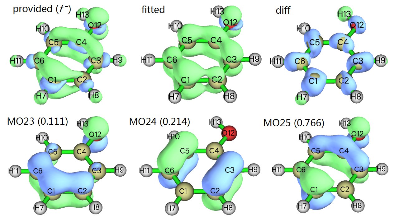
From the map above, it can be seen that our fitted grid data is very close to the provided one, at least the fitted one is able to reasonably reproduce the basic character in π region. The main difference between the provided and the fitted grid data is the σ region, as clearly reflected in the "diff" subgraph. This observation implies that loss of an electron causes severe relaxation of σ electrons, which cannot be fully represented based on the occupied MOs of N-state.
The MO23, MO24 and MO25 shown in the map above are all π orbitals, this fact explains why the σ part of the \(f^-\) cannot be faithfully represented in the fitted grid data. Notice that a few MOs have negative contributions, the one with most negative value is MO20 (-0.108). If you check this orbital, you will find it is an σ orbital. However, since its shape is not quite similar to the "diff" grid data, its existence does not improve the fitting quality or lower the difference between the provided and fitted grid data.
From the map above we can also find the profile of isosurface of MO25 is very similar to the \(f^-\), this is why MO25 has dominant contribution and also why \(f^-\) can often be reasonably approximated by HOMO distribution. It is obvious that if there is no orbital relaxation effect, contribution of MO25 should be exactly 1.0 while all other MOs should have contribution of 0.0.
Note
It is worth to stress that the range of the orbital considered in the fitting affects the resulting contributions. For example, you only want to calculate contribution of MOs 10~15, you will find their contributions are different when MOs 1~15 are chosen and when MOs 10~15 are chosen.
4.200.13.2 Contribution of NBO orbitals to Fukui function f− of 1,3-butadiene
This time we calculate contribution of various highly occupied NBOs to \(f^-\) of 1,3-butadiene. The .fch file of N and N-1 states, as well as NBO plot files .31 and .37 generated for N state have been provided in "examples\orb_densdiff\butadiene" folder. The geometry has been optimized for N-state.
Note that the NBO orbitals recorded in the .37 file can be divided into two categories, the Lewis type and Rydberg type. The Lewis NBOs have an occupation number of approximately 2.0 while the Rydberg ones are almost unoccupied. Since only the Lewis NBOs significantly contribute to electron density of N-state, we will only take these orbitals into account.
First, we generate cube file of \(f^-\) type of Fukui function. Boot up Multiwfn and input
examples\orb_densdiff\butadiene\butadiene.fch
5 // Calculate grid data
0 // Set custom operation
1 // Only one file will be operated with the file that has been loaded
-,examples\orb_densdiff\butadiene\butadiene_N-1.fch
1 // Electron density
1 // Low-quality grid (since the current system is very small, low-quality grid is adequate)
2 // Export the grid data as density.cub in current folder
Now reboot Multiwfn and input
examples\orb_densdiff\butadiene\BUTADIENE.31
37 // Load the BUTADIENE.37 in the same folder, which records NBO orbitals
Now if you enter main function 6 and choose option 3 to examine orbital information, you will find the first 15 orbitals correspond to Lewis type of NBOs due to their high occupation numbers. Next, we input below commands in the main menu
200 // Other functions (Part 2)
13 // Evaluate orbital contributions to density difference or other grid data
density.cub // The file containing grid data of \(f^-\)
0 // Choose orbital range and start analysis
1-15 // Range of Lewis NBOs
The result is shown below
 Orbital     3   Value:    -0.047
 Orbital     8   Value:    -0.046
[ignored...]
 Orbital    10   Value:     0.017
 Orbital     4   Value:     0.530
 Orbital     9   Value:     0.531
 Sum of all values:       1.000
 Fitting error (definition 1):      0.9008
 Fitting error (definition 2):    0.004961
The data clearly shows that NBO4 and NBO9 equally and fully dominate the \(f^-\), while participation of other orbitals can be safely ignored.
The isosurface (isovalue=0.01) of the provided \(f^-\) and the fitted one, as well as isosurface (isovalue=0.1) of NBO4 and NBO9 are collectively shown below
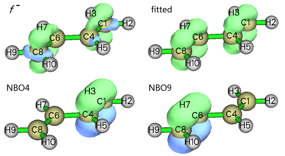
Since from the graph it is obvious that NBO4 and NBO9 correspond to π bond of C1-C4 and C6-C8, respectively, and the fitted function is qualitatively consistent with the provided \(f^-\), we can conclude that the \(f^-\) is mainly composed of the π electrons over the C1-C4 and C6-C8 bonds.
4.200.13.3 Contribution of NBO orbitals to density difference between S0 and S1 states of H2CO
Finally, we study contribution of NBOs to Δρ between S1 and S0 states of H2CO.
All relevant files used in this section have been provided in "examples\orb_densdiff\H2CO" folder, including the NBO plot files generated for ground state, wavefunction file of ground state (S0.fch) and wavefunction of the first excited state (S1.wfn). The Gaussian input files used for generating these files are also provided.
We first generate the Δρ between S1 and S0 states. Boot up Multiwfn and input
examples\orb_densdiff\H2CO\S1.wfn
5 // Calculate grid data
0 // Set custom operation
1 // Only one file will be operated with the file that has been loaded
-,examples\orb_densdiff\H2CO\S0.fch
1 // Electron density
1 // Low-quality grid
2 // Export the grid data as density.cub in current folder
-1 // Visualize the isosurface
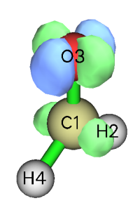
The isosurface at isovalue=0.03 is shown below.
examples\orb_densdiff\H2CO\H2CO.31
37 // Load the H2CO.37 in the same folder, which records NBO orbitals
200 // Other functions (Part 2)
13 // Evaluate orbital contributions to density difference or other grid data
density.cub // The file containing grid data of ΔρS0→S1
1 // Set constraint on the sum of contributions
2 // Set the constraint to a specific value
0 // Since electron excitation does not alter the number of electrons, the sum of contributions is set to be constrained to zero
0 // Choose orbital range and start analysis
[Press ENTER button to consider all orbitals] // Note that during electron excitation, a portion of electrons is excited to empty orbitals, therefore only taking Lewis NBOs into account is evidently inadequate, so all orbitals should be taken into account in the present context
The result is shown below
 Orbital     8   Value:    -0.719
 Orbital    16   Value:    -0.254
 Orbital     9   Value:    -0.151
[ignored...]
 Orbital    11   Value:     0.115
 Orbital    22   Value:     0.132
 Orbital    18   Value:     0.148
 Orbital    32   Value:     0.894
 Sum of all values:       0.000
 Fitting error (definition 1):      0.4778
 Fitting error (definition 2):    0.001770
It can be seen that the NBO having dominant positive value is NBO32. The NBO having the most negative contribution is NBO8, its magnitude of negative contribution is by far greater than any other NBO. From the "Natural Bond Orbitals (Summary)" field printed by NBO module in the Gaussian output file examples\orb_densdiff\H2CO\S0.out, it can be seen that the NBO8 is identified as " LP ( 2) O 3", namely lone pair of O3.
The isosurface of fitted Δρ (isovalue=0.03) as well as isosurface of NBO8 and NBO32 (both isovalues are set to 0.17) are shown below.
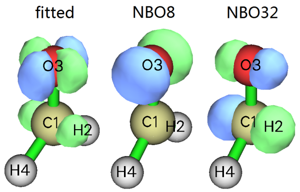
By comparing the "fitted" graph with the ΔρS0→S1 graph shown earlier, it is apparent that the fitted Δρ is almost completely identical to the rigorously calculated one, hence the fitting quality in the current instance is fairly high and the contribution values must be very reliable and meaningful. From the orbital isosurface maps it is obvious that the NBO8 indeed corresponds to lone pair of O3, while NBO32 corresponds to anti-π orbital of C1-O3, therefore the S0→S1 excitation could be unambiguously identified as n(O3)→π*(C1-O3) type of transition.
You can also calculate contribution of various NAOs to the S0→S1 excitation, the only difference from the example above is that after loading the H2CO.31, you should input 33 to load the H2CO.33, which records NAO orbitals. You will find the S0→S1 excitation mainly involves transitions from highly occupied p type NAOs to those nearly unoccupied.
4.200.14 Domain analysis examples
The domain analysis refers to quantitative analysis for the region enclosed by isosurface of given real space function, see Section 3.200.14 for details. To illustrate the powerfulness and flexibility of the domain analysis module, some practical applications of the domain analysis are given below.
4.200.14.1 Integrate real space functions within reduced density gradient (RDG) isosurface to study weak interaction quantitatively
Before reading this, please read Section 3.23.1 to understand how to use reduced density gradient (RDG) to reveal weak interaction regions. In this section, I show the possibility of characterizing weak interaction by integrating domains enclosed by RDG isosurfaces.
System 1: Phenol dimer
First, we use phenol dimer as example. Boot up Multiwfn and input
examples\phenoldimer.wfn
200 // Other functions (Part 2)
14 // Integrate real space functions within isosurfaces of a real space function
Here we want to study RDG domains defined as regions enclosed by isosurface of RDG = 0.5; in other words, these domains are composed of grid points where RDG < 0.5. Therefore, we select option 2 and choose "13 Reduced density gradient", and then select option 3 and input criterion, namely <0.5 (In fact, RDG < 0.5 is the default setting and you do not need to manually do these steps). Next, input below commands:
1 // Start calculation grid data and generate domains
-10 // Adjust extension distance
0 // Set extension distance to zero to avoid wasting of grid points at boundary area, where RDG isosurfaces commonly do not occur
2 // Medium-quality grid (grid spacing=0.1 Bohr), generally this is accurate enough
Now Multiwfn starts calculation of grid data for the selected real space function (i.e. RDG), and then identifies individual RDG domains according to the criterion of RDG<0.5. Finally, four domains are found, the number of grid points constituting the domains are shown as the last column:
Domain:     1    Grids:     208    Volume:     0.031 Angstrom^3
Domain:     2    Grids:     290    Volume:     0.043 Angstrom^3
Domain:     3    Grids:     200    Volume:     0.030 Angstrom^3
Domain:     4    Grids:    2597    Volume:     0.385 Angstrom^3
To visualize them, select "3 Visualize domains". In the GUI, you can select domain index at right-bottom list. The 2nd and 4th domains are shown below:
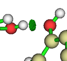
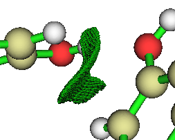
If you have read Section 3.23.1, you must know these domains correspond to H-bond and van der waals (vdW) interactions between the two phenols, respectively. We can study properties of these domains in terms of integrating specific real space functions within corresponding regions. We input
1 // Integrate a domain
2 // Index of the domain of interest
2 // Choose a real space function
1 // Using electron density as integrand
the result is:
 Integration result:    0.6932973049E-02 a.u.
 Volume:    0.290000 Bohr^3  (    0.042974 Angstrom^3 )
 Average:    0.2390680362E-01
 Maximum:    0.2766231164E-01   Minimum:    0.1994457517E-01
Similarly, we do this for domain 4:
 Integration result:    0.1181667175E-01 a.u.
 Volume:    2.597000 Bohr^3  (    0.384836 Angstrom^3 )
 Average:    0.4550123895E-02
 Maximum:    0.6217203920E-02   Minimum:    0.3102088666E-02
From the output we know the number of electrons involved in the domains corresponding to H-bond and vdW interactions are 0.006933 and 0.011817, respectively. They can be interpreted as overlapping electrons and are closely related to strength of same type of interactions. However, since these two domains correspond to different types of weak interactions, the magnitude of overlapping electrons is not positively correlated to their strengths, namely we are unable thus to conclude that the vdW interaction between the two phenols is stronger than the intermolecular H-bond. The "Volume" in the output denotes volume of the domain, we can find that vdW interaction involves much wider spatial region than H-bond. "Average" corresponds to average value of real space function in the domain, from this quantity one can easily infer that the strength of interaction per contact region of H-bond must be significantly higher than that of vdW interaction, since as shown above, their average values are 0.0239 and 0.0045, respectively, the former is much larger than the latter.
System 2: 2-pyridoxine 2-aminopyridine
Intermolecular H-bonds of 2-pyridoxine 2-aminopyridine (PP) have been investigated in Section 4.2.1 by means of AIM analysis, while this time we will analyze them by means of \(q_{\mathrm{int}}\) index. This index was proposed in J. Phys. Chem. A, 115, 12983 (2011) for judging interaction of H-bond at various intermolecular distance, please check Section 3.200.14 for its definition. Commonly, the more negative of the \(q_{\mathrm{int}}\) index, the more stable the interaction.
\(q_{\mathrm{int}}\) index is defined based on integrating domains enclosed by RDG = 0.6 isosurfaces, therefore we need to first calculate RDG grid data and generate corresponding domains. Note that it is not always appropriate to set extension distance of RDG grid data to zero. For present system, if you calculate RDG grid data by main function 5 with extension distance of zero, you will see some RDG isosurfaces are truncated by box boundary, as shown below and highlighted by red arrows. In this case the domain-integration module of Multiwfn does not work.
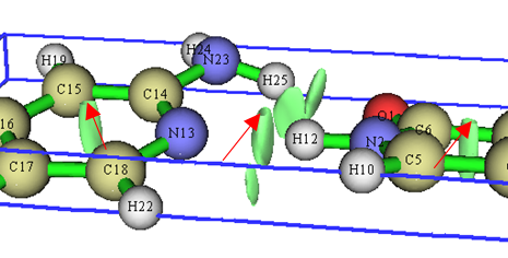
Therefore, when we calculate RDG grid data for this case, extension distance should be set somewhat larger than zero, 3 Bohr is safe enough for avoiding unexpected truncation. Extension distance should also never be set to an over-large value, otherwise the number of grid points to be calculated will be very high and thus very time-consuming.
Boot up Multiwfn and input below commands:
examples\2-pyridoxine_2-aminopyridine.wfn
200 // Other functions (Part 2)
14 // Integrate real space functions within isosurfaces of a real space function
3 // Change the default criterion of defining domain
<0.6
1 // Start calculation of grid data
-10 // Change extension distance
3 // 3.0 Bohr of extension distance
2 // Medium-quality grid
Now visualize resulting domains. Domains 2 and 4 are shown below, clearly they correspond to H-bond of N23-H25⋅⋅⋅⋅⋅⋅O1 and N2-H12⋅⋅⋅⋅⋅⋅N13, respectively.
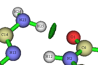
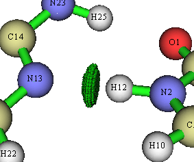
Next, select option "5 Calculate q_bind index for a domain" and input 2, then press ENTER button directly to use ρ4/3 as the integrand (which was used in J. Phys. Chem. A, 115, 12983 (2011)), the resulting \(q_{\mathrm{int}}\) and related details of the domain are shown below
 q_att:       0.00490957 a.u.
 q_rep:       0.00005590 a.u.
 q_bind:     -0.00485367 a.u.
 Volume (lambda2<0):     0.599000 Bohr^3
 Volume (lambda2>0):     0.010000 Bohr^3
 Volume (Total):         0.609000 Bohr^3
Similarly, we obtain results for domain 4
 q_att:       0.00805204 a.u.
 q_rep:       0.00037346 a.u.
 q_bind:     -0.00767858 a.u.
 Volume (lambda2<0):     0.745000 Bohr^3
 Volume (lambda2>0):     0.052000 Bohr^3
 Volume (Total):         0.797000 Bohr^3
Since the \(q_{\mathrm{bind}}\) corresponding to N2-H12⋅⋅⋅⋅⋅⋅N13 (-0.007678) is much more negative than that of N23-H25⋅⋅⋅⋅⋅⋅O1 (-0.004854), the former should be stronger than the latter.
Since both the interactions are H-bond, it is also possible to simply compare the number of electrons contained in the domains to estimate their relative strength. We choose "2 Perform integration for all domains", then input 2, and then select electron density as integrand to obtain electron population of all domains:
Domain    Integral (a.u.)     Volume (Bohr^3)      Average
     1    0.1212147834E-03         0.111000    0.1092025076E-02
     2    0.1647945811E-01         0.609000    0.2705986553E-01
     3    0.1714432107E-02         0.319000    0.5374395319E-02
     4    0.2618188584E-01         0.797000    0.3285054685E-01
     5    0.8932587581E-02         0.412000    0.2168103782E-01
     6    0.7764521413E-02         0.394000    0.1970690714E-01
 Integration result of all domains:    0.6119409984E-01 a.u.
 Volume of all domains:     2.642000 Bohr^3       0.391504 Angstrom^3
Not only the integration value of domain 2 (0.01648) is evidently smaller than domain 4 (0.02618), but also the average value of domain 2 (0.02706) is smaller than domain 4 (0.03285), therefore we have strong evidence to say N2-H12⋅⋅⋅⋅⋅⋅N13 is stronger than N23-H25⋅⋅⋅⋅⋅⋅O1.
With similar steps illustrated in this section, you can also integrate other real space functions such as potential energy density and spin density in the domains enclosed by isosurfaces of other real space functions, e.g. IRI, δ\(g^{\mathrm{inter}}\) and ELF.
Note that the accuracy of integration in the domains is directly determined by grid setting, higher quality of grid leads to better accuracy. For example, when visualizing domains, if you found a domain only consists of very few grid points, and its profile is very coarse, then integration accuracy of this domain must be very low.
4.200.14.2 Visualize molecular cavity and calculate its volume by domain analysis module
This is an application instance of domain analysis module, I will briefly illustrate how to use Multiwfn to visualize molecular cavity and calculate cavity volume. More examples and information about this topic can be found in my blog article “Using Multiwfn to visualize molecular cavity and calculate cavity volume” (http://sobereva.com/408, in Chinese).
The idea of using domain analysis to study molecular cavity is very simple: We first calculate promolecular density, then we define the regions having electron density lower than a threshold e.g. 0.0001 as molecular cavity. More than one such regions may exist, the domain analysis module automatically assigns them with different domain indices. After that, by visualizing the domains, it should be easy to find the domain corresponding to the molecular cavity. The choice of threshold is somewhat arbitrary, commonly 0.001~0.0001 a.u. is appropriate.
α-cyclodextrin is used as an example in this section. Before studying the cavity using domain analysis module, it is suggested to first visualize promolecular density under various isovalues. Boot up Multiwfn and input:
examples\alpha-cyclodextrin.pdb
5 // Calculate grid data
1 // Promolecular density
-10 // Set extension distance
0 // Zero extension distance, namely let the box just enclose the molecule
1 // Low-quality grid
-1 // Show isosurface map
Click "Show data range" in the GUI window to show the box of grid data as blue frame, and set isovalue to 0.01 and 0.001 respectively, you will see
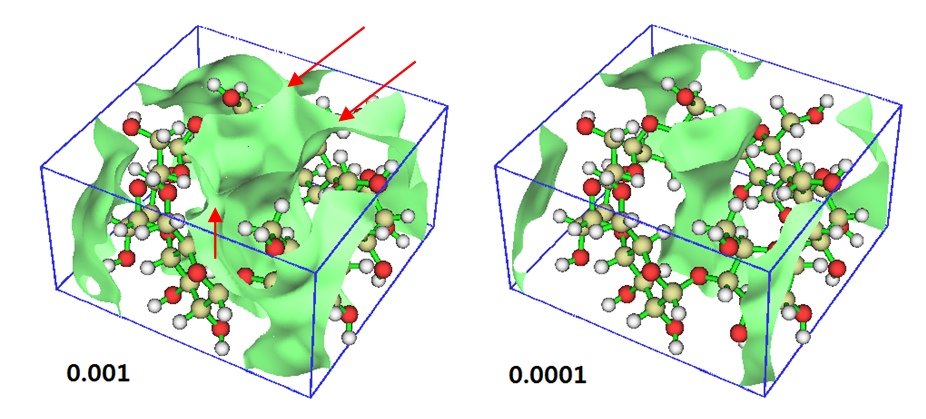
It is easy to understand, if we use threshold of 0.001 a.u., then the domain corresponding to the cavity in the center of the molecule cannot be defined, because the internal region and external region are connected via the three channels pointed by red arrows. While in the case of 0.0001 a.u., the molecular cavity is clearly identifiable and thus we could use domain analysis module with this threshold to study the cavity.
Return to main menu, and then input below commands
200 // Other functions (Part 2)
14 // Domain analysis
2 // Choose the real space function to be calculated and used for partitioning domains
1 // Promolecular density
3 // Define the rule of determining domains
<0.0001 // Regions with electron density less than 0.0001 will be defined as domains
1 // Calculate grid data and assign domains
-10 // Change extension distance
0 // No extension distance
1 // Low-quality grid
After calculation is finished, you will see the following information on screen. There are totally six domains found, the number of grids and volume of all domains are shown
Domain:     1    Grids:       4    Volume:     0.005 Angstrom^3
Domain:     2    Grids:   12010    Volume:    14.238 Angstrom^3
Domain:     3    Grids:    5822    Volume:     6.902 Angstrom^3
Domain:     4    Grids:   39654    Volume:    47.009 Angstrom^3
Domain:     5    Grids:   13949    Volume:    16.536 Angstrom^3
Domain:     6    Grids:    7438    Volume:     8.818 Angstrom^3
Then we can visualize each domain by option 3. After examining the domains, we find that the domain with index of 4 is the one corresponding to molecular cavity, as shown below:
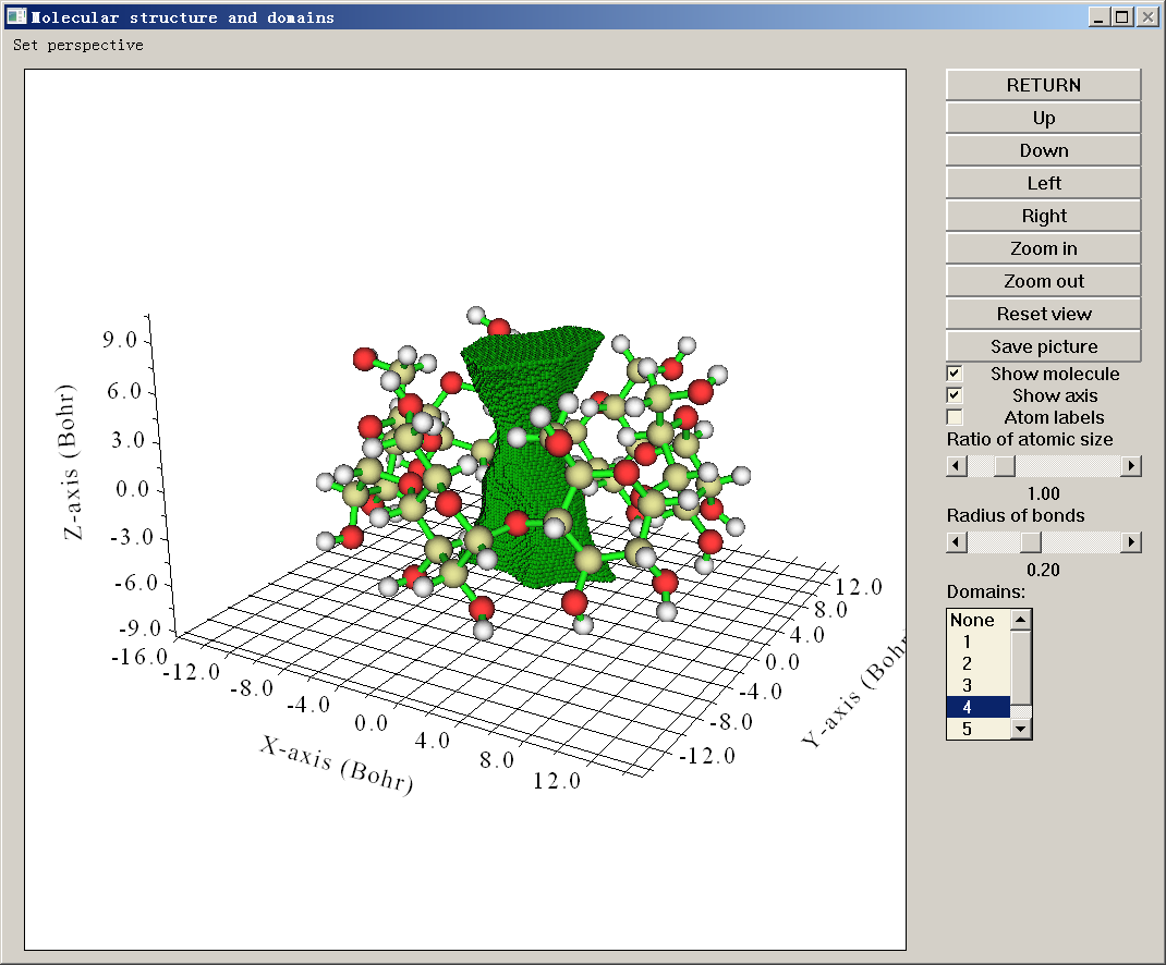
Since this domain well represents shape of actual molecular cavity, its volume is a good indicator of cavity size. As shown earlier, its volume is 47.0 Å3.
Close the GUI, select option 1 to carry out integration within domain, and input 4 to choose to integrate the domain corresponding to the cavity. We choose "100 User-defined real space function" as integrand (by default, this function is 1.0 everywhere and thus does not take any computational cost), then the following information is printed on screen
Integration result:    0.3172320000E+03 a.u.
 Volume:  317.232000 Bohr^3  (   47.008943 Angstrom^3 )
 Average:    0.1000000000E+01
 Maximum:    0.1000000000E+01   Minimum:    0.1000000000E+01

 Position statistics for coordinates of domain points (Angstrom):
 X minimum:   -2.7823  X maximum:    3.1445  Span:    5.9268
 Y minimum:   -2.6823  Y maximum:    2.6095  Span:    5.2918
 Z minimum:   -3.1770  Z maximum:    3.9140  Span:    7.0910
The integration result directly corresponds to the volume of the domain (47.0 Å3) since the current integrand is 1.0 everywhere, from the output we also find the span distance of the domain, in Z direction the value is 7.09 Å, which is the difference between the points in the domain with maximum Z and with minimum Z coordinates. So, using Multiwfn we can not only obtain cavity volume but also obtain cavity span distance.
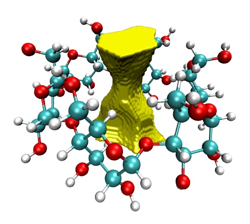
Furthermore, we can export a selected domain as domain.cub in current folder by using option 10, so that the domain can be portrayed as isosurface in third-part visualization tools, such as VMD. In the resulting domain.cub, the grids within the selected domain have value of 1, while grids in other regions (as well as boundary grids) have value of 0, therefore isosurface of domain can be rendered with isovalue between 0 and 1 (commonly 0.5 is used). We do this for the domain 4 and plot it as isosurface in VMD, the graph below will be obtained
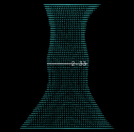
We can also use option 11 to export boundary grids of a domain to domain.pdb, in which each particle corresponds to a boundary grid. You can load this file into VMD and render the particles as points. Then if you want to measure domain, you can click keyboard button 2, then click two points in the graphical window, the linking line will appear and the distance will be labelled, as illustrated below ("Display" - "Orthographic" was selected for easier inspection)
4.200.14.3 Integrate electron density difference in its isosurfaces
In this section, we integrate electron density difference (EDD) in its isosurfaces. Specifically, the EDD in this section corresponds to deformation density (Δρdef), see Section 3.7.2 for its definition. Benzene is taken as instance.
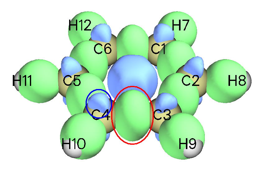
The .cub file of EDD for benzene (benzene_EDD.cub) has been provided at http://sobereva.com/multiwfn/extrafiles/benzene_EDD.zip. You can also easily generate it using main function 5. We first examine its isosurface map. Boot up Multiwfn and load benzene_EDD.cub, then enter main function 0, set isovalue to 0.015, you will see the following map. The green and blue isosurfaces correspond to positive and negative parts, respectively, which correspond to electron density increase and decrease regions due to formation of benzene from isolated atoms. In this example, we will use domain analysis module to respectively integrate the EDD within the two domains indicated by the red and blue circles.
Return to main menu, and then input
200 // Other functions (Part 2)
14 // Domain analysis
3 // Set criterion for defining domain
<-0.015 // The regions with function value more negative than -0.015 will be determined as domains, which is in line with the blue isosurfaces shown above
-1 // Yield domains based on the grid data in memory
Domains are immediately generated:
Domain:      1    Grids:     1912    Volume:     0.8502 Angstrom^3
Domain:      2    Grids:      433    Volume:     0.1925 Angstrom^3
Domain:      3    Grids:      423    Volume:     0.1881 Angstrom^3
Domain:      4    Grids:      434    Volume:     0.1930 Angstrom^3
Domain:      5    Grids:      432    Volume:     0.1921 Angstrom^3
Domain:      6    Grids:      430    Volume:     0.1912 Angstrom^3
Domain:      7    Grids:      427    Volume:     0.1899 Angstrom^3
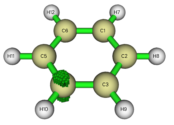
Enter option 3 to visualize the domains. By checking distribution of every domain, we find domain 3 corresponds to the blue isosurface mentioned above, as shown below. Each small green sphere corresponds to a grid within the domain.
Then we integrate EDD within domain 3. Close the GUI window and input
1 // Perform integration for a domain
3 // Domain index is 3
1 // The integrand is just the grid data in memory, namely EDD
The result is -0.032 a.u.
Next, we integrate EDD within the green isosurface mentioned earlier. Input:
0 // Exit domain analysis module
14 // Domain analysis
3 // Set criterion for defining domain
>0.015
-1 // Yield domains based on the grid data in memory
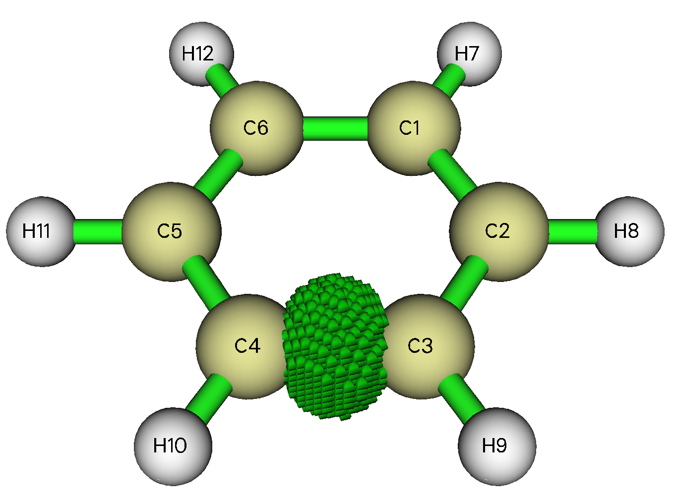
After visually checking, we find domain 14 corresponds to the isosurface of interest, as shown below
Close the GUI window and input
1 // Perform integration for a domain
14 // Domain index is 14
1 // The integrand is just the grid data in memory, namely EDD
The result is 0.156 a.u.
Finally, it is worth to emphasize that because the integral is evaluated numerically based on uniform grids, the smaller the grid spacing, the better the integration accuracy.
You can similarly integrate other kinds of EDD, including Fukui function and dual descriptor.
4.200.18 Studying bond length/order alternation (BLA/BOA) as well as alteration of bond angle and dihedral for specific paths
Note
Chinese version of this section is my blog article “Using Multiwfn to calculate bond length/order alternation (BLA/BOA) and study variation of bond length, bond order and angle with respect to bond index” (http://sobereva.com/501), which contains more discussion.
The basic knowledge about definition and calculation of bond length alternation (BLA) and bond order alternation (BOA) have been introduced in Section 3.200.18. Multiwfn can not only calculate BLA and BOA, but can also calculate variation of bond length, bond order, bond angle and dihedral along a given path. This function is quite useful in studying characteristics of conjugated chains. In this section two examples will be given.
In this function, any file format that carries geometry information can be used as input file, such as .xyz, .pdb and .mol. However, if you also want to study BOA, the input file must contain basis function information, such as .mwfn, .fch, .molden or .gms.
4.200.18.1 BLA and BOA of thiophene oligomer
In this section, we will calculate BLA and BOA for a thiophene oligomer with 5 repeat units, the .fchk file generated at PBE0/6-31G* level can be downloaded here: http://sobereva.com/multiwfn/extrafiles/TP5.zip. The geometry was optimized at B3LYP/6-31G* level.
Before calculation, you need to first determine indices of the atoms in the conjugated chain of interest. The easiest way of doing this is using GaussView. Now we use GaussView (version ≥ 6.0) to open the TP5.fchk, choose  button in the "Builder" panel, then hold down the left mouse button and let the cursor pass through each atom in the conjugated chain to select them as yellow. After that, the image in the GaussView window should look like this:
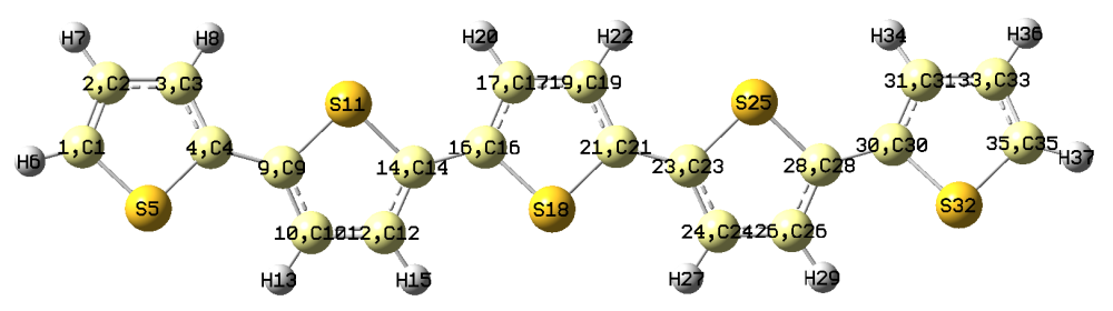
Then enter "Tools" - "Atom Selection", you will find the atom indices of the selected chain is 10,12,14,16-17,19,21,23-24,26,28,30-31,33,35. Also, as can be seen from the above figure, the index of the atom at the beginning side and ending side is 1 and 35, respectively.
Note
Of course, it is not absolutely necessary to use GaussView for the present function. However, without GaussView, you have to manually record indices of all atoms in the chain by means of visual inspection, obviously this process is fairly troublesome!
Now boot up Multiwfn and input
TP5.fchk
200 // Other functions (Part 2)
18 // Calculate bond length/order alternation (BLA/BOA) and study variation of bond characteristics with respect to bond index
10,12,14,16-17,19,21,23-24,26,28,30-31,33,35 // The indices of the atoms in the chain
1,35 // Index of the atom at the beginning side and ending side
Then Multiwfn automatically identifies the atom sequence of the chain based on your inputted information. As can be seen from screen, the identified sequence is
Sequence of the atoms in the chain from the beginning side to the ending side
       1       2       3       4       9      10      12      14      16
      17      19      21      23      24      26      28      30      31
      33      35
If you compare the sequence with the graph of molecular structure, you will find the sequence is completely correct, therefore the subsequent data should be meaningful.
Next, the bond index, indices of the two atoms composing the bond, bond length and bond order are given:
  Bond     Atom1     Atom2   Length (Angstrom)   Mayer bond order
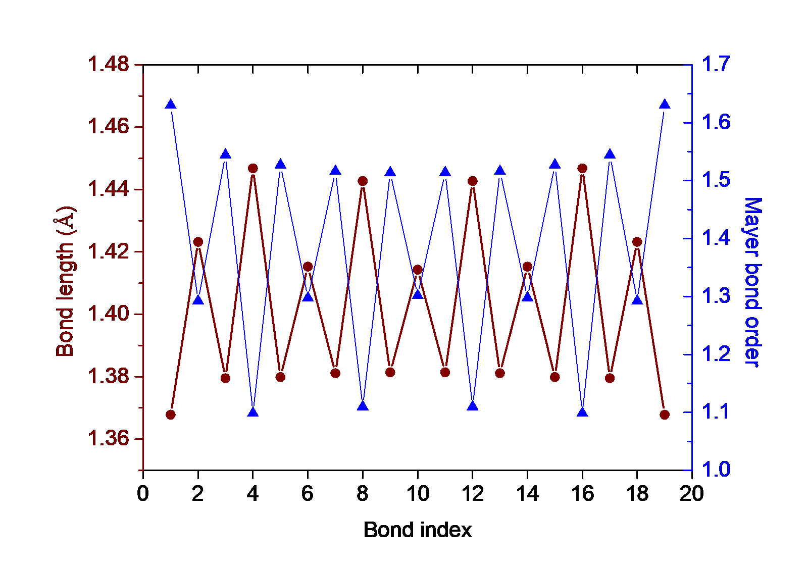
     1         1         2        1.3678              1.6303
     2         2         3        1.4232              1.2924
     3         3         4        1.3795              1.5445
     4         4         9        1.4468              1.0985
     5         9        10        1.3799              1.5273
[ignored...]
Finally, some statistical data as well as BLA and BOA are shown:
 The number of even bonds:     9
 The number of odd bonds:     10
 Average length of even bonds:       1.4300 Angstrom
 Average length of odd bonds:        1.3779 Angstrom
 Bond length alternation (BLA):      0.0521 Angstrom
 Average bond order of even bonds:      1.2109
 Average bond order of odd bonds:       1.5465
 Bond order alternation (BOA):         -0.3356
As mentioned on the screen, the bond data have also been exported to bondalter.txt in current folder, you can plot "bond length vs. bond index" and "bond order vs. bond index" curve maps. The map below was plotted by Origin, the corresponding .opj file has been provided as bondalter.opj in "examples" folder.
Multiwfn also asks you if outputting variation of bond angle and dihedral along the atom sequence, we input n because they are not what we are currently interested in.
4.200.18.2 Study variation of bond lengths, bond angles and dihedrals in the ring of cyclo[18]carbon
The map below is a frame of ab-initio molecular dynamic trajectory of the cyclo[18]carbon at 200 K. This simulation was conducted in my research article Chem. Asian J., 16, 56 (2021) DOI: 10.1002/asia.202001228. In this section we will study variation of bond lengths, bond angles and dihedrals along the ring.
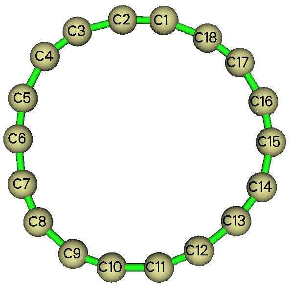
Boot up Multiwfn and input
examples\C18_MD_1.xyz // A frame extracted from molecular dynamics trajectory
200 // Other functions (Part 2)
18
1-18 // The atom indices in the ring
1,1 // The path under study is a closed path, i.e. a ring, in this case the two inputted atom indices must be the same. Index of any atom in the ring could be inputted, it will be regarded as the beginning atom
The outputted bond length variation is shown below
  Bond     Atom1     Atom2   Length (Angstrom)
    1         1         2         1.208
    2         2         3         1.375
    3         3         4         1.209
[...ignored]
   17        17        18         1.201
   18        18         1         1.384
Next, we input y to let Multiwfn output variation of bond angles and dihedrals along the defined path, you will see:
Note The unit of printed values is degree

 Atoms:     1     2     3  Angle:   164.841
 Atoms:     2     3     4  Angle:   154.976
 Atoms:     3     4     5  Angle:   155.200
[...ignored]
 Atoms:    17    18     1  Angle:   162.906
 Atoms:    18     1     2  Angle:   158.520

 Atoms:     1     2     3     4  Dihedral:  28.69, deviation to planar:  28.69
 Atoms:     2     3     4     5  Dihedral:  25.51, deviation to planar:  25.51
 Atoms:     3     4     5     6  Dihedral:  22.98, deviation to planar:  22.98
[...ignored]
 Atoms:    17    18     1     2  Dihedral:  16.91, deviation to planar:  16.91
 Atoms:    18     1     2     3  Dihedral:  18.13, deviation to planar:  18.13
From the above output we can easily examine how bond angles and dihedrals vary along the 18-membered ring. Note that the value range of dihedral (D) is 0~180°, the "deviation to planar" is identical to D if the D is within 0~90°, while it corresponds to 180−D if the D is within 90~180°.
If you copy the data from screen (see Section 5.4 if you do not know how to do this) and plot them via external software such as Origin, you can obtain the following maps, which very clearly exhibit geometric characteristics of the ring:
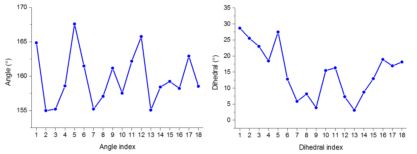
Since bond angles and dihedrals fluctuate evidently along the ring, we can conclude that the ring undergoes prominent geometry deformation during the molecular dynamics simulation.
4.200.19 Examples of calculating spatial delocalization index
Please read Section 3.200.19 to understand basic knowledge of spatial delocalization index (SDI). In this example we will calculate SDI for density of orbital wavefunctions to characterize spatial delocalization extent of various orbitals. SDI can also be applied to quantify spatial delocalization of any other function, such as spin density.
Note that the ODI described in Section 4.8.5 is also able to compare orbital delocalization extents; however, definitions of ODI and SDI are different, and SDI is in principle more rigorous and free of choice of atom partition method.
Calculate SDI based on wavefunction file
As an example, we calculate SDI for densities of all occupied orbitals of examples\excit\D-pi-A.fchk. Boot up Multiwfn, load this file, and then input
200 // Other function (Part 2)
19 // Calculating SDI
2 // Calculate SDI for density of orbital wavefunctions
1-56 // Indices of occupied MOs
You will immediately see following result on screen, the unit is a.u.
...ignored
SDI of orbital    11:    0.3763
SDI of orbital    12:    0.5834
SDI of orbital    13:    0.5287
SDI of orbital    14:    0.4195
SDI of orbital    15:    0.3759
SDI of orbital    16:    0.3759
SDI of orbital    17:    4.9640
SDI of orbital    18:    4.5899
SDI of orbital    19:    6.0700
SDI of orbital    20:   11.5668
...ignored
You can use such as Origin to plot SDI value versus orbital index:
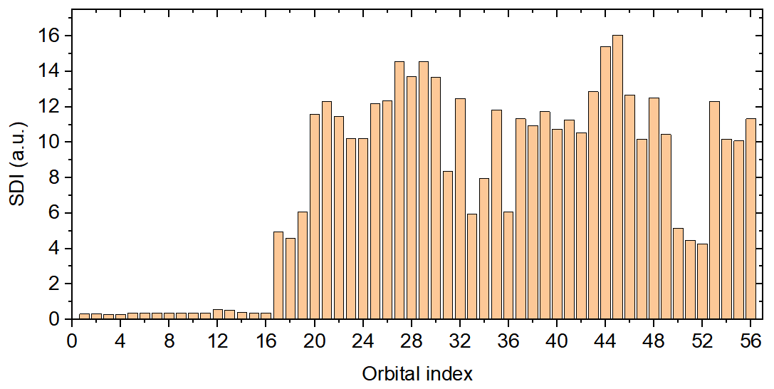
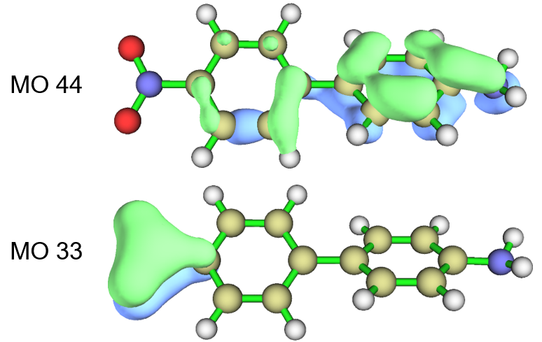
The larger the SDI of an orbital density, the more evident the orbital delocalization character. From the map above, you can infer that orbital 44 is strongly delocalized (SDI = 15.41 a.u.), while orbital 33 (SDI = 5.97 a.u.) is highly localized. See the following map for comparison. Orbitals from 1 to 16 are evidently core orbitals since they show extreme localization character, as indicated by the extremely low SDI.
Calculate SDI based on grid data file
To calculate SDI, you can not only provide a file containing wavefunction information as input file, but can also provide a grid data file (e.g. cube file) containing the function to be studied. As an example, we calculate SDI based on grid data of density of MO19 of the D-pi-A system, the file can be downloaded at http://sobereva.com/multiwfn/extrafiles/D-pi-A_MO19_dens.zip. Boot up Multiwfn and load the cube file in the compressed package, then input
200 // Other function (Part 2)
19 // Calculating SDI
3 // Calculate SDI based on grid data in memory
Then you will see:
This result is in good agreement with the SDI of MO19 computed based on examples\excit\D-pi-A.fchk, which is 6.07.
Sometimes the quantum chemistry or first-principles program that can produce grid data file cannot generate a wavefunction file that supported by Multiwfn, in this case if you need to calculate SDI to study orbital delocalization, you have to calculate SDI based on grid data file like this example.
Multiwfn can also be used to calculate SDI of any other function as long as it is natively supported by Multiwfn or you can provide a grid data file of that function. For example, if you use cube file recording spin density as input file and input the same commands as the present example, then the resulting SDI can be used to characterize spatial extent of delocalization of spin density.
4.200.20 Using bond order density and natural adaptive orbital to study chemical bonds
Note
Chinese version of this topic is "Using bond order density (BOD) and natural adaptive orbital (NAdO) to graphically study chemical bonds" (http://sobereva.com/535), which contains much more examples and fuller discussions.
The theory of bond order density (BOD) and natural adaptive orbital (NAdO) has been detailedly introduced in Section 3.200.20, please carefully read it first. In this section I will present two examples to show how to use the BOD and NAdO to study chemical bonds.
4.200.20.1 Plot bond order density for N2 molecule
The delocalization index (DI) represents average number of electron pairs shared by two atoms and can be regarded as a definition of (covalent) bond order. By plotting BOD, we can better understand the nature of its value. The integral of the BOD defined for two atoms over the whole space exactly corresponds to the DI between the two atoms, therefore BOD is able to exhibit local contributions everywhere to DI.
N2 molecule is taken as example in the present section, we will plot its BOD as color-filled map in the molecular plane. In Multiwfn, delocalization index (DI) can be calculated based on fuzzy partition via fuzzy atomic space analysis module (main function 15) or based on atom-in-molecules (AIM) partition via basin analysis module (main function 17); correspondingly, both the two modules can export atomic overlap matrix (AOM), which is needed by BOD analysis. In the present example, we use the former (the latter works equally well but more expensive).
Boot up Multiwfn and input below commands
examples\N2.fch // Optimized and generated at B3LYP/def-TZVP level. You can also use other files (e.g. .molden and .mwfn) as long as the file contains basis function information
15 // Fuzzy atomic space analysis
3 // Calculate and output atomic overlap matrix to AOM.txt in current folder
0 // Return to main menu
200 // Other functions (Part 2)
20 // Bond order density (BOD) and natural adaptive orbital (NAdO) analyses
1 // Use atomic overlap matrix (AOM) for the analysis
[Press ENTER button] // Load the AOM.txt in current folder
1,2 // Indices of the two atoms to be analyzed
Then NAdOs are generated and you can find the following information
Generating natural adaptive orbitals (NAdOs)...
Eigenvalues of NAdOs: (sum=   3.11681 )
  1.00000   0.99999   0.99999   0.05728   0.05728   0.00113   0.00113
The values are eigenvalues of the NAdO orbitals, the sum (3.11681) just corresponds to the DI between the two atoms. At the same time, NAdOs.mwfn is generated in current folder, in which the first 7 orbitals are the NAdO orbitals, their occupation numbers correspond to the NAdO eigenvalues. All other orbitals in this file are identical to the virtual MOs in the N2.fch.
Next, we input y to let Multiwfn load the newly generated NAdOs.mwfn. From now on, electron density function directly corresponds to the BOD function. Now we plot the BOD as color-filled map. Input below commands
0 // Return to main menu
4 // Plot plane map
1 // Electron density (which corresponds to BOD in the present context)
1 // Color-filled map
[Press ENTER button] // Use recommended grid setting
0 // Set extension distance
2 // 2 Bohr
3 // YZ plane
0 // Z=0
Now the BOD map pops up. After some adjustments on plotting settings, you can see the map below
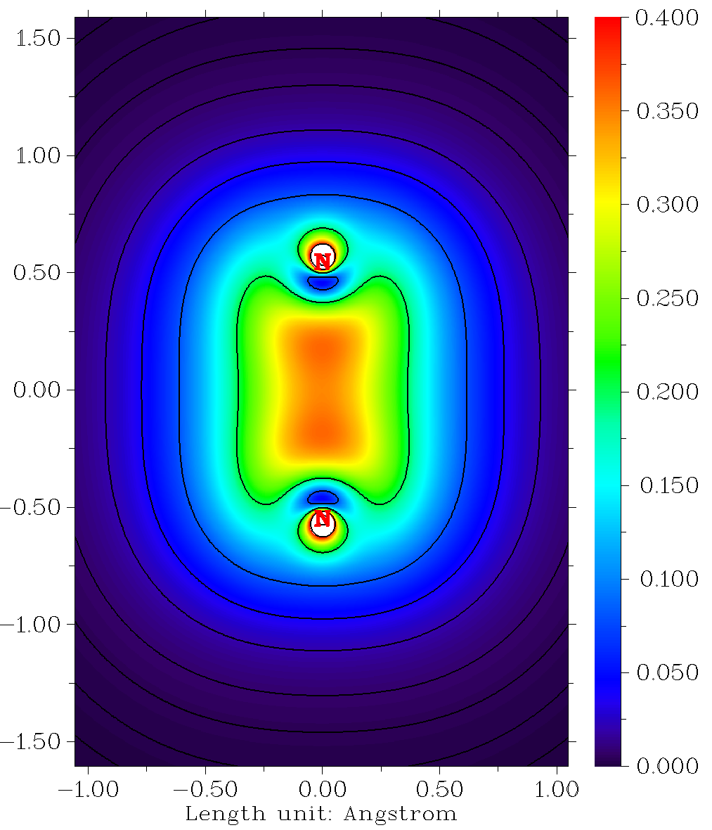
It can be seen that the distribution of BOD is reasonable, its main body is distributed in the bonding area, showing that the electrons in this region have major contribution to the DI value and play crucial role in the covalent bond.
4.200.20.2 Study BOD and NAdO orbitals for C-C bonds in butadiene
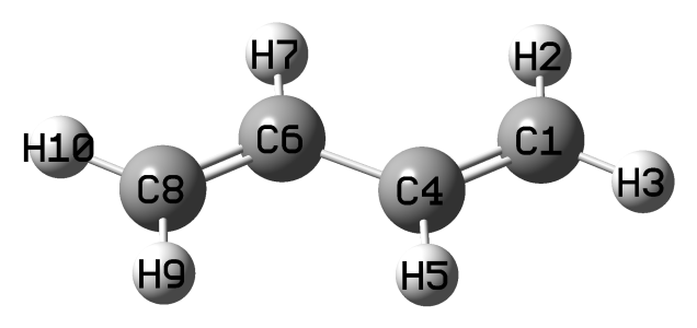
In this section, we will study BOD and NAdO orbitals for two kinds of C-C bonds in 1,3-butadiene, whose geometry is shown below. This time the analysis will be performed based on the AOM generated by AIM partition (using fuzzy partition like the last example is also reasonable).
Boot up Multiwfn and input
examples\butadiene.fch // Generated at B3LYP/6-31G** level
17 // Basin analysis module
1 // Generate basins and locate attractors
1 // Use electron density to define basins (i.e. AIM basins)
2 // Medium-quality grid
6 // Output orbital overlap matrix in atoms to AOM.txt in current folder
-10 // Return to main menu
200 // Other functions (Part 2)
20 // Bond order density (BOD) and natural adaptive orbital (NAdO) analyses
1 // Use atomic overlap matrix (AOM) for the analysis
[Press ENTER button] // Load the AOM.txt in current folder
4,6 // Indices of the two carbons at the center of the system
Now you can see
Eigenvalues of NAdOs: (sum=   1.11455 )
   0.90121   0.24533   0.07666   0.00358   0.00062   0.00006   0.00001
   0.00000  -0.00000  -0.00003  -0.00004  -0.00316  -0.00966  -0.02645
  -0.07359
That means the DI of the central C-C bond is 1.114. Then input y to load the newly generated NAdOs.mwfn file. After that, we use main function 5 to calculate grid data of electron density, which now corresponds to BOD, and then plot it as isosurface. The resulting map with isovalue of 0.05 is shown below.
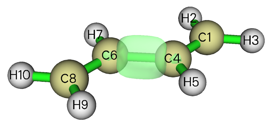
It is obvious that most electrons that have significant contribution to the C4-C6 bond are concentrated around this bond, this is what we expected.
Next, enter main function 0 to visualize various NAdO orbitals. Note that if you select "Orbital info." - "Show all" in the GUI menu, you can see below orbital information
 Orb:     1 Ene(au/eV):     0.000000       0.0000 Occ: 0.901215 Type:A+B (?   )
 Orb:     2 Ene(au/eV):     0.000000       0.0000 Occ: 0.245331 Type:A+B (?   )
 Orb:     3 Ene(au/eV):     0.000000       0.0000 Occ: 0.076660 Type:A+B (?   )
 Orb:     4 Ene(au/eV):     0.000000       0.0000 Occ: 0.003580 Type:A+B (?   )
 Orb:     5 Ene(au/eV):     0.000000       0.0000 Occ: 0.000621 Type:A+B (?   )
[...ignored]
 Orb:    14 Ene(au/eV):     0.000000       0.0000 Occ:-0.026445 Type:A+B (?   )
 Orb:    15 Ene(au/eV):     0.000000       0.0000 Occ:-0.073586 Type:A+B (?   )
 Orb:    16 Ene(au/eV):    -0.023511      -0.6398 Occ: 0.000000 Type:A+B (?   )
 Orb:    17 Ene(au/eV):     0.084006       2.2859 Occ: 0.000000 Type:A+B (?   )
 Orb:    18 Ene(au/eV):     0.115938       3.1548 Occ: 0.000000 Type:A+B (?   )
[...ignored]
The first 15 orbitals are NAdOs, their "Occ" values correspond to NAdO eigenvalues, which can be regarded as contribution of the NAdOs to DI. All orbitals with index larger than 15 are the virtual MOs in the examples\butadiene.fch, they are not of our interest. From the above list, it can be seen that only the first two NAdO orbitals have prominent contribution to DI, their isosurface maps are shown below, the eigenvalues are also labelled.
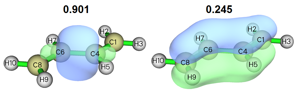
It can be seen that the first NAdO, which looks like a σ type of localized orbital (see example in Section 4.19.1 for more information about this point), has key contribution (0.901) to the DI value (1.114); this is fully understandable, since the major ingredient of the C4-C6 bond must be σ interaction. The second NAdO also has nonnegligible contribution (0.245). Since it shows typical π orbital character, we can infer that weak π interaction exists in the C4-C6 bond.
Now we turn our attention to the boundary C-C bonds, namely C1-C4 (or C6-C8). Reboot Multiwfn and input below commands (you can first manually backup the previous NAdOs.mwfn to avoid overwriting)
examples\butadiene.fch
200 // Other functions (Part 2)
20 // Bond order density (BOD) and natural adaptive orbital (NAdO) analyses
1 // Use atomic overlap matrix (AOM) for the analysis
[Press ENTER button] // Load the AOM.txt in current folder
1,4 // Indices of the two carbons at the boundary of the system
y // Load the newly generated NAdOs.mwfn
After that, use main function 0 to visualize the only two orbitals having significant contributions to DI, as shown below (isovalue=0.05)
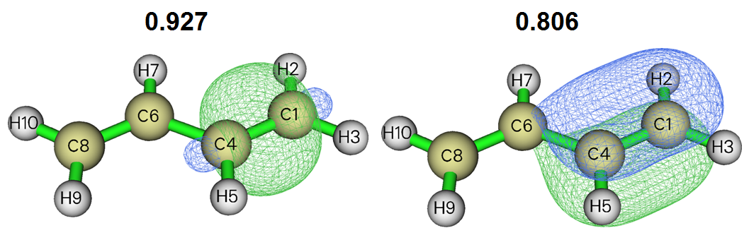
The σ type of NAdO orbital of C1-C4 has comparable eigenvalue to that of C4-C6, indicating that both kinds of C-C bonds have similar strength of σ interaction. In contrast, the π type of NAdO orbital of C1-C4 has much higher contribution to DI than that of C4-C6, well reflecting the fact that the boundary C-C bonds have much stronger π interaction than the central one.
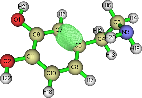
At the end of this section, I would like to emphasize a quite noteworthy point of the BOD/NAdO method, namely you can directly specify the bond to be studied, as already fully illustrated above. For example, for the dopamine shown below, if you want to study BOD or corresponding NAdOs for a bond, e.g. C5-C7, you simply need to input 5,7 when Multiwfn asks you to input atom indices, clearly this feature makes bonding analysis quite convenient! The following map shows BOD=0.03 isosurface for C5-C7.
Also, it is noteworthy that the BOD/NAdO analysis can also be performed to visualize DI between two basins based on the BOM.txt exported by basin analysis module. For example, you can use basin analysis module to generate electron localization function (ELF) basins and then export basin overlap matrix (BOM) to BOM.txt by corresponding option. After that, in the BOD/NAdO analysis function, select to load the BOM.txt, and then input index of two basins of interest, the NAdOs for the two local regions will be generated. Via this manner, you can visually study e.g. electron sharing between two lone pair regions or between a lone pair and a covalent bonding region. Clearly, the BOD/NAdO analysis module is extremely flexible!
4.200.20.3 Study interaction between two fragments using BOD/NAdO
I also extended BOD and NAdO analyses to the scenario of interfragment interaction. To illustrate how to realize this, in this section I take oxirane as an example molecule, the oxygen atom and the two carbon atoms will be respectively defined as the two fragments. In addition, in this example I will illustrate evaluation of energies for NAdOs.
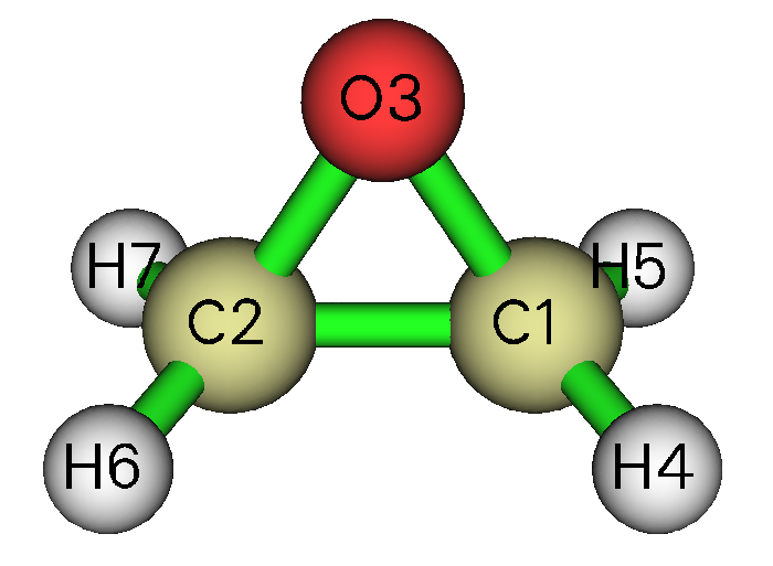
We generate a file containing AOMs as previous examples. Boot up Multiwfn and input
examples\oxirane.fchk
15 // Fuzzy atomic space analysis
3 // Calculate and output atomic overlap matrix to AOM.txt in current folder
0 // Return to main menu
200 // Other functions (Part 2)
20 // Bond order density (BOD) and natural adaptive orbital (NAdO) analyses
-1 // Toggle if calculating energies for NAdOs
1 // Evaluate NAdOs energies based on the Fock matrix generated by MO energies and coefficients
3 // Interfragment interaction analysis based on fragment overlap matrix (FOM)
[Press ENTER button] // Load AOM.txt in current folder
3 // Fragment 1: The oxygen atom
1,2 // Fragment 2: The two carbons
The loaded AOMs are used to construct FOMs of the two fragments, the eigenvalues of generated NAdOs are
Eigenvalues of NAdOs: (sum=   2.47514 )
  0.97214   0.86882   0.35986   0.10399   0.08304   0.03930   0.02916
  0.02059   0.00045   0.00042   0.00013  -0.00275
As can be seen, there are three NAdO orbitals having notable contributions to DI. In addition, as shown in the prompt on screen, energies of NAdOs are evaluated in this case.
After inputting y to load the newly generated NAdOs.mwfn in current folder, you can visualize their isosurfaces in main function 0, as shown below. The eigenvalues and energies are also labelled:
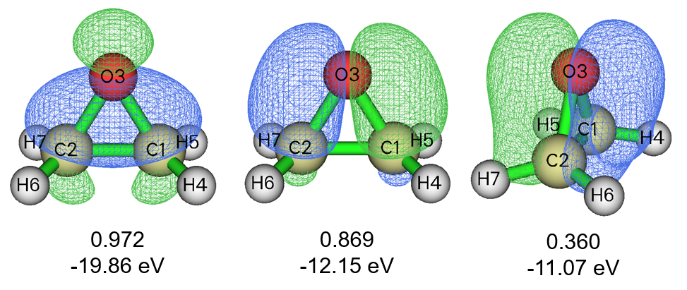
It is obvious that the above three NAdO orbitals nicely elucidated the orbital interaction between fragment O1 and fragment C1-C2, and in the interacting region the same phase overlap can be clearly observed. Among them, the first NAdO has the lowest energy, indicating that it has the largest contribution to the interfragment binding. Please then plot BOD map in the plane defined by C1, C2 and O3 via main function 4 to visualize distribution of the electrons directly contributing to the interfragment interaction.
This is only a very simple example showing the usefulness of BOD/NAdO of revealing interfragment interaction, evidently it can also be applied to much more complicated situations to gain deeper insights, such as the interaction between the iron atom and the two cyclopentadienyl rings in ferrocene, the interaction between encapsulated atom and cage in atomic cluster.
Finally, I also would like to mention that in the fuzzy atom space analysis module, you can use option -1 to switch the space partition method to Hirshfeld-I before generating AOM file; in some cases, especially when metal is involved, the result may be notably better than using the default partition.