4.6 Modify and check wavefunction

4.6.1 Delete certain Gaussian functions

In subfunction 25 of main function 6, you can set orbital expansion coefficients of Gaussian type functions (GTFs) which satisfy certain conditions. If the coefficients are set to zero, that means the information of these GTFs are deleted. In this example, we delete all Z-type GTFs of atoms 2, 3 and 4 from orbital 23 of phenol and then plot isosurface for this molecular orbital. Boot up Multiwfn and input following commands

examples\phenol.wfn
6  // Modify wavefunction
25  // Set the coefficients of some GTFs that satisfied certain conditions
0,0  // Set the index range of GTFs, only the GTFs satisfied this condition will be reserved to next step. 0,0 tell Multiwfn the range is “ALL”
2,4  // Only the GTFs attributed to atoms 2, 3, 4 will be reserved to next step
Z  // Only reserve Z-type GTFs to next step
23,23  // Set lower and upper limit of orbital, if they are identical, then only one orbital is selected
0  // Set coefficients of selected GTFs in orbital 23 to zero, that is delete their information
0  // Save current wavefunction to new.wfn in current directory

You can choose option 4 and input 23 to check expansion coefficient of orbital 23 to verify if your operation is correct. Let us compare the isosurfaces of orbital 23 before and after modification. In order to plot the modified orbital 23, you can close Multiwfn and load new.wfn, or directly select option -1 to return to the main menu, and then enter main function 0 to plot its isosurface.

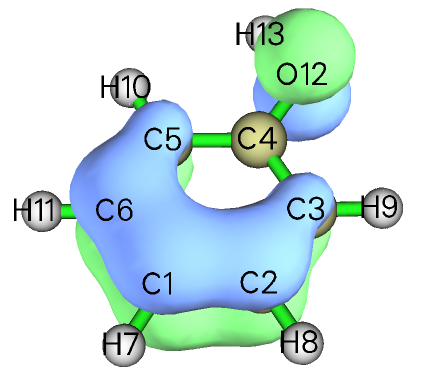
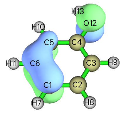
Left side is unmodified state, the molecular plane is parallel to XY plane, so if Z-type GTFs in some atoms are deleted, the corresponding part of isosurface should disappear, this is what we have seen at right side (modified state).

4.6.2 Valence electron density analysis: Example of removing contributions from certain orbitals to real space functions

In Multiwfn, contributions from certain orbitals to real space functions can be removed. From the formulae in Section 2.6 it is clear that if occupation numbers of certain orbitals are set to zero, they will have no contribution, as if they do not exist. Actually, in Section 4.5.3 we have already used this trick to separate ELF as ELF-σ and ELF-π. Notice that some real space functions are not linear with respect to orbitals, such as ELF and LOL, so they cannot be computed as the sum of contributions from each occupied orbital. In contrast, some real space functions are linear with respect to orbitals, such as electron density and kinetic energy density, they can be decomposed as contributions from various orbitals.

If we study electron density after removing contributions from inner-core molecular orbitals, then the analysis is known as “valence electron density analysis”, which was demonstrated to be quite powerful for analyzing molecular electronic structure. Lots of examples of this kind of analysis can be found in my paper "Revealing Molecular Electronic Structure via Analysis of Valence Electron Density" Acta Phys. -Chim. Sin., 34, 503 (2018) DOI: 10.3866/PKU.WHXB201709252.

Next, two examples of studying valence electron density are given.

Example 1: Plotting color-filled map of valence electron density for HCN

In this example, we will manually remove contributions from the MOs consisting of inner-core atomic orbitals to electron density for HCN, so that we can plot its valence electron density map, the procedure is very simple. Inner-core atomic orbitals always have very low energy, so they can only contribute to the MOs with lowest energy. Hydrogen has no inner-core atomic orbital, while both carbon and nitrogen have an inner-core atomic orbital, hence what we need to do is to set occupation numbers of the first two MOs to zero (note that this is closed-shell wavefunction).

Now, boot up Multiwfn, and input following commands

examples\HCN.wfn
6  // Modifying wavefunction
26  // Set occupation numbers
1,2  // Select MOs 1 and 2
0  // Set their occupation numbers to zero
q  // Return to last menu
-1  // Return to main menu

Then, if we plot color-filled map of electron density as usual by main function 4 (see examples in Section 4.4), we will get the following graph

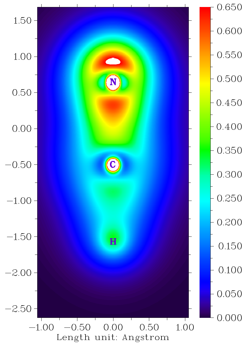
From the above picture, the bonding region of C-N and C-H bonds and be easily identified, and the lone pair region of nitrogen can also be clearly observed. Note that the small white circles in carbon and nitrogen centers do not correspond to 1s electrons, but result from the fact that valence atomic orbitals have penetration effect into core region.

Example 2: Plotting isosurface map of valence electron density for ethane

For convenience consideration, Multiwfn provides option 34 in main function 6, one can directly choose it to set occupations of all MOs composed of inner-core atomic orbitals to zero. In this example we will use this feature, and plot isosurface map of valence electron density for ethane.

Boot up Multiwfn and input

examples\ethane.wfn
6  // Modify wavefunction
34  // Set occupation number of inner orbitals to zero
-1  // Return to main menu
5  // Calculate grid data and visualize isosurface map
1  // Electron density
3  // High-quality grid
-1  // Show isosurface map

After changing isovalue to a proper value 0.25 and disable showing molecular structure, we will see

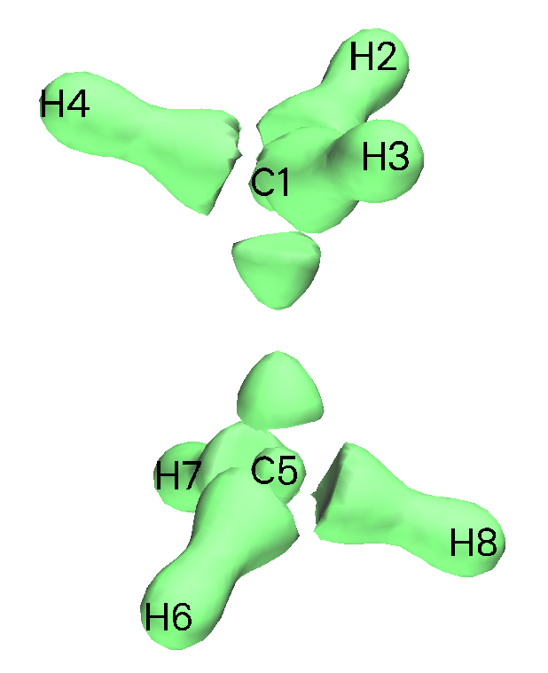
As you can see, the core electrons of carbon, as well as the electrons used to form C-C bond and C-H bonds, are clearly revealed by the isosurfaces.

Finally, it is worth to mention that analysis of valence electron density is never limited to plotting analysis. For example, by using main functions 2 and 17, topology analysis and basin analysis can also be straightforwardly applied to valence electron density, respectively; what you need to do is removing contributions of inner-core MOs (as illustrated above) before performing usual analysis for electron density.

See my blog article “Studying direction of nucleophilic attack via electron localization function (ELF) and valence electron density analysis” (http://sobereva.com/606, in Chinese) on more examples about valence electron density analysis.

4.6.3 Translate and duplicate graphene primitive cell wavefunction to periodic system

Note

IMPORTANT NOTE: To analyze wavefunction for periodic system, it is best to use Multiwfn in combination with CP2K, see Section 2.9.2. The main purpose of this section is simply illustrating the features of translating and duplicating wavefunction.

The .fch or .wfn file generated by periodic boundary condition (PBC) calculation of Gaussian only contains wavefunction of primitive cell, so the analysis results do not show any periodic character, of course you can expand your system to multiple cells before PBC calculation, but you have to spend much more time for computation. Multiwfn provides a way to convert primitive cell wavefunction to a large supercell wavefunction, so that in the region of interest, the real space functions show periodic character.

Note

Beware that constructing supercell wavefunction in this manner is only a very crude approximation! Since the orbital mix between neighbouring primitive cells is ignored, therefore the orbital wavefunctions of supercell cannot be faithfully reproduced.

In this section I use graphene as example. First, generating .fch (or .wfn) file of graphene primitive cell. The content of “molecular specification” field in the Gaussian input file is

C                  0.000000    0.000000    0.000000
C                  0.000000    1.429118    0.000000
TV                 2.475315    0.000000    0.000000
TV                -1.219952    2.133447    0.000000

In route section, write “#P PBEPBE/3-21g/Auto SCF=Tight”. Use Gaussian to run this input file and then use formchk to convert the binary checkpoint file to graphene.fch. Then boot up Multiwfn and input:

examples\graphene.fch
6  // Modify wavefunction
32  // Translate and duplicate primitive cell wavefunction
2.475315,0.0,0.0  // Translation vector 1
2  // Unit is Å
3  // Translate and duplicate present system three times in this direction
32  // Notice that current system already has four primitive cells, this time we will translate and duplicate current system in another direction three times, so the final system will contain 16 primitive cells
-1.219952,2.133447,0.0  // Translation vector 2
2  // Unit is Å
3  // Translate and duplicate present system three times in this direction

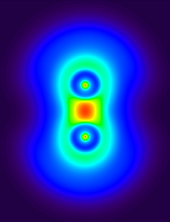
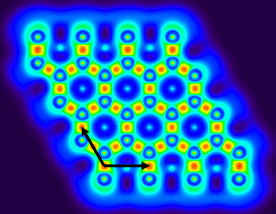
The left part of the picture below is LOL function of primitive cell. After above manipulation, we recalculate LOL function and then the right graph is obtained (black arrows denote translation vectors). Apparently, the central region of the extended system shows correct periodic character, however the behavior of boundary region is still incorrect, you can extend the system further to enlarge “correct” region.

Notice that if nosymm keyword is not specified in PBC calculation, Gaussian may automatically put the system into standard orientation, at this time you should not use the translation vectors in Gaussian input file as the translation vectors for translating and duplicating system in Multiwfn, but should use the content in “Translation vectors” field of .fch file or “PBC vector” segment in Gaussian output file.