3.100 Other functions, part 1 (100)

Since Multiwfn has too many functions, some of the functions are relatively "small" compared to main functions, and some functions are not closely related to wavefunctions analysis, these functions are classified as "other functions". Because the number of subfunctions in "other functions" are huge, "other functions" are split as part 1 (main function 100) and part 2 (main function 200). Part 1 will be described below, and part 2 will be introduced in Section 3.200.

3.100.1 Draw scatter graph between two functions and generate their cube files

This function allows grid data of two functions to be generated at the same time with sharing grid setting, you can choose to export their cube files, view their isosurfaces and plot scatter graph between them.

After you entered this function, select two real space functions that you are interested in, for example you want to analyze real space functions 16 and 14, you should input 16,14 (the first and the second function will be referred to as functions 1 and 2 respectively below). Then select a mode to set up grid points. After that Multiwfn starts the calculation of grid data for them. Once the calculation is finished, Pearson correlation coefficient of the two functions in all grid points is printed and a menu appears on screen, all options are self-explanatory. If you choose -1 to draw scatter graph, a graph like this will pop up immediately:

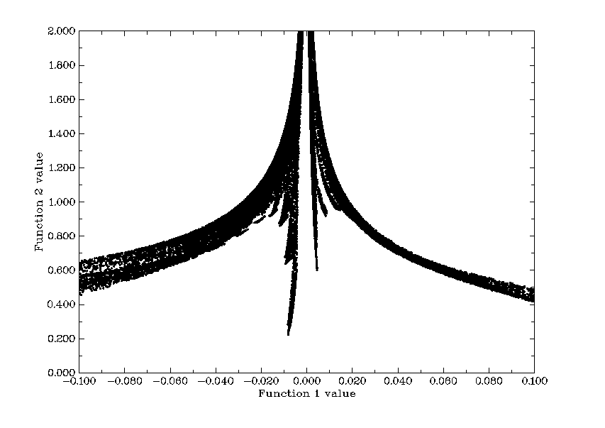
Each scatter point corresponds to each grid point, the position in X-axis and Y-axis corresponds to the value of function 1 and function 2 at this point, respectively. Multiwfn determines the range of axes automatically according to the minimum and maximum value, sometimes you have to use option 4 and 5 to reset the range yourself, otherwise barely points can be seen in the graph. The size of points can be adjusted by “symbolsize” in settings.ini. The graph can be saved to current directory by option 1. The X-Y data set of the points can be exported to output.txt in current directory by option 2.

Option -2 and -3 set the value of function 2 where the value of function 1 is within or without of a specific range respectively. Notice that the data once modified cannot be retrieved again.

Special usage: If you already have cube files of the two functions to be studied (referred to as func1.cub and func2.cub, respectively) and you want to directly use the functions in post-processing menu (e.g. plotting scatter map, modifying values), you should follow these steps: Input the path of func1.cub after booting up Multiwfn, then enter main function 100 and select subfunction 1, then input 0,0 when selecting real space functions, then input the path of func2.cub, after that the grid data of the two cube files will be directly taken as function 1 and function 2. Notice that, of course, the grid setting of func1.cub and func2.cub must be exactly identical.

3.100.2 Export various files or generate input file of quantum chemistry programs

Exporting various kinds of files

This function can be used to output current structure to .pdb, .xyz, .gro, .cif, .cml files. Wavefunction information can be exported as .wfn or .wfx file when only GTF information is available, and can also be exported as .mwfn, .molden, .fch, GENNBO input file (.47), old Molekel input file (.mkl) when basis function information is presented. Clearly, Multiwfn can be used as a very useful file format converter, e.g. .mwfn/.wfn/.wfx/.fch/.molden/.gms ... → .pdb/.xyz/.cml/.gjf/.wfn/.wfx/.molden/.fch/.47 ...

In addition, it is worth to note that one can use Gaussian or other codes to generate .fch or .molden file, then use Multiwfn to convert it to .mkl file, and then use orca_2mkl test -gbw to convert test.mkl to test.gbw, so that ORCA can use wavefunction generated by other codes as initial guess. I also have a shell script to automate this procedure, see http://sobereva.com/517.

If current input file is .chg format, which carries atom information and atomic charges (see Section 2.5 for details), you can use option 1 to convert it to .pqr file. The .pqr and .pdb formats are very similar, the major differences is that the former has additional two columns to record atomic charges and atomic radii. In the resulting .pqr file, the atomic charges are identical to that in .chg file, while the atomic radii column corresponds to Bondi vdW radii. The .pqr can be directly loaded into VMD program, the atoms can be colored according to atomic charges (if the fourth column of .chg file records other atomic information such as atomic spin populations, in VMD the atoms can also be colored according to spin populations). This is very useful for intuitively exhibiting atomic properties, see Section 4.A.10 for illustrations.

Exporting grid data file

When there is a set of grid data in memory (may be loaded from e.g. .cub file or calculated by e.g. main function 5), then:

• Via option 35 you can export the popular .cub file.

• Via option 36 you can export .vti file, which is a format supported by the well-known and freely available volume data visualizer ParaView (https://www.paraview.org), also at the meantime Multiwfn asks you if also exporting a .cml file recording current system with Bohr as unit, if you choose to export it, you can use ParaView to load it so that grid data and molecule structure can be simultaneously plotted.

• Via option 37 you can export grid data in VASP format, just like CHGCAR and LOCPOT.

Generating input file of quantum chemistry and first-principles programs

This function is also able to yield the input file for a batch of known quantum chemistry codes based on current structure, net charge and multiplicity, including Gaussian, GAMESS-US, ORCA, MOPAC, Dalton, MRCC, Molpro, NWChem, PSI4, CFOUR, Molcas. Input files of a popular first-principles codes CP2K and Quantum ESPRESSO can also be generated.

For generating Gaussian or GAMESS-US input file, if basis function information is presented, you can select if writing the orbital expansion coefficients to their input files so that the present wavefunction can be used as initial SCF guess. Notice that you must then manually specify the basis set in the input file as the one originally used to yield present wavefunction, otherwise the Gaussian or GAMESS-US task must be failed.

When exporting Dalton input files, if basis function information is presented, you can choose to write orbital expansion coefficients to the exported .dal file, which can be directly used as initial guess. Via this design, for example, you can easily use the unrestricted natural orbitals (UNO) generated from a UHF/UKS wavefunction as initial orbitals for CASSCF calculations of Dalton (Dalton itself does not support UHF/UKS!). See “Using Multiwfn to take orbitals generated by other programs as initial guess in Dalton calculations” (in Chinese, http://sobereva.com/740) for detailed information and examples.

Because ORCA is very popular, fast and has numerous important functions, while its keywords are not as easy to specify as Gaussian, therefore a special interface is provided for generating ORCA input file, in which commonly employed ORCA calculation levels can be selected, the generated keywords are the most appropriate and efficient ones for corresponding level. Very detailed description can be found in "On the function of generating ORCA input file in Multiwfn "(in Chinese, http://sobereva.com/490), also there is an practical example "Simulating UV-Vis and ECD spectra using ORCA and Multiwfn" (http://sobereva.com/485). The video "Study geometry, vibration, IR spectrum and orbitals based on ORCA program and other codes" (https://youtu.be/tiTmTbtbtig) also utilized this function.

Because PSI4 code is very popular in performing symmetry-adapted perturbation theory (SAPT), the function of generating PSI4 input file was elaborately designed for this purpose.

The ability of generating CP2K input file is extremely powerful and useful. After loading a geometry file of molecular or periodic system into Multiwfn, this function is able to generate CP2K input file of various tasks with wide variety of frequently used options. See "Using Multiwfn to very conveniently create input file of CP2K" (http://sobereva.com/587) for detail.

Information needed

Atom coordinates, GTFs (for exporting .wfn/.wfx), basis functions (for exporting .mwfn/.fch/.molden/.47), grid data (for export cub, vti and VASP grid data)

3.100.3 Calculate molecular van der Waals volume

In this function Monte Carlo method is used for evaluating van der Waals (vdW) volume of present system, two definitions of vdW region are provided: (1) The superposition of vdW sphere of atoms. This definition is not very accurate, because electron effect is not taken into consideration, but the speed of evaluation is very fast and wavefunction information is not required. (2) The region encompassed by certain isosurface of electron density, the isovalue of 0.001 is suitable for isolated system, while 0.002 is more suitable for molecules in condensed phase. One can choose the definition by "MCvolmethod" in settings.ini.

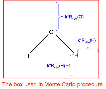
The principle of the Monte Carlo procedure is very simple: If we define a box (volume is \(L\)) which is able to hold the entire system, and let \(N\) particles randomly distributed in the box, if \(n\) particles are presented in the vdW region, then the vdW volume of present system is \(n/N\ast L\). Of course, the result improves with the increase of \(N\). In Multiwfn, you need to define \(N\) by input a number \(i\), the relationship is \(N=100\times 2^{i}\), for small molecular when \(i\)=9 the accuracy is generally acceptable, for large system you may need to increase \(i\) gradually until the result variation between \(i\) and \(i+1\) is small enough to be acceptable as converged. For definition 2 of vdW region, you also need to input the isovalue of density, and the factor \(k\) used to define the box, see below illustration, where R_vdw is vdW radius. If \(k\) is too small, then the vdW region may be truncated, however if \(k\) is too large, more points are needed to maintain enough accuracy. For isovalue of 0.001, \(k\)=1.7 is recommended.

Information needed

atom coordinates (for definition 1), GTFs (for definition 2)

3.100.4 Integrate a function over the whole space

This is a very useful and powerful function for integrating selected real space function in the whole space. The numerical integration method used here is based on the one proposed by Becke in the paper J. Chem. Phys., 88, 2547 (1988) for integrating DFT functional, which is also suitable for any real space function, but notice that the function must be smooth and converges to zero at infinite asymptotically. The accuracy is determined by the number of integration points, you can adjust the number of radial and angular integration points by “radpot” and “sphpot” parameters in settings.ini, respectively. The integrand can be selected from built-in functions, and you can also write new function yourself as user-defined function, see Sections 2.6 and 2.7.

If outmedinfo in settings.ini is set to 1, then during the calculation of this function, a file named integrate.txt will be exported in current folder, which contains these data for all integrating points: Index, Cartesian coordinate, function value, Lebedev integration weighting, and atom weighting function.

Examination of difference of a real space function between two wavefunction files

By the way, if you would like to examine difference between two wavefunction files for a real space function, you can select function -4 or -5 (hidden functions) in main function 100, the function to be integrated will be [\(f\)(file1)-\(f\)(file2)]² or |\(f\)(file1)-\(f\)(file2)|, respectively, where \(f\) is the real space function you will select, “file1” is the wavefunction file loaded when Multiwfn boots up, and “file2” is the wavefunction file you will choose in this function. In this function you can also set criterion of electron density and thus let Multiwfn only evaluate the difference for low density region (i.e. ignoring core region). In addition, after calculation, Multiwfn automatically exports grid data of file1 as a plain text file in current file, the file name directly reflects current calculation condition. For example, the file name a.wfn_003_0075_0434 implies that “file1” is a.wfn, the 3rd real space function was selected, the radial and angular integration points are 75 and 434, respectively. In later studies, if all calculation conditions match with the file name (the file must be placed in current folder), then Multiwfn will directly load data of “file1” from this file rather than recalculate them to reduce computational time.

Evaluation of spherically symmetric average ELF / LOL

In J. Comput. Chem., 38, 2258 (2017), the authors proposed that the optimal ω parameter of range-separated DFT functionals can be determined by means of below quantity:

\[\begin{gathered}r_{\mathrm{ELF}}=\sqrt{\frac{\int \mathrm{ELF}(\mathbf{r})r^2\mathrm{ELF}(\mathbf{r})\mathrm{d}\mathbf{r}}{\int \mathrm{ELF}(\mathbf{r})\mathrm{ELF}(\mathbf{r})\mathrm{d}\mathbf{r}}}\end{gathered}\]

In Multiwfn, this quantity will be automatically calculated and outputted if you select ELF as the integrand in present function. The \(r_{\mathrm{ELF}}\) is outputted as “spherically symmetric average ELF”, the numerator and denominator in the root sign are also outputted together.

In J. Phys. Chem. C, 123, 4407 (2019), the LOL-tuning is proposed, in which the “spherically symmetric average LOL” is involved:

\[\begin{gathered}r_{\mathrm{LOL}}=\sqrt{\frac{\int \mathrm{LOL}(\mathbf{r})r^2\mathrm{LOL}(\mathbf{r})\mathrm{d}\mathbf{r}}{\int \mathrm{LOL}(\mathbf{r})\mathrm{LOL}(\mathbf{r})\mathrm{d}\mathbf{r}}}\end{gathered}\]

The \(r_{\mathrm{LOL}}\) along with its numerator and denominator in the root sign will be printed if LOL is selected in present function.

An example is given in Section 4.100.4.

Information needed

Atom coordinates, GTFs.

3.100.5 Show overlap integral between alpha and beta orbitals

For unrestricted wavefunctions, the orthonormalization condition does not in general hold between alpha and beta orbitals. This function computes the overlap matrix between alpha and beta orbitals

\[\begin{gathered}S_{i,j}^{\alpha\beta}=\int \varphi_{i}^{\alpha}(\mathbf{r})\varphi_{j}^{\beta}(\mathbf{r})\mathrm{d}\mathbf{r}\end{gathered}\]

The diagonal elements are useful for evaluating the matching degree of corresponding spin orbital pairs, evident deviation to 1 indicates that spin polarization is remarkable.

In present function, there are two options, option 1 calculates the full overlap matrix, the diagonal elements will be printed on screen and the whole overlap matrix can be selected to output to ovlpmat.txt in current folder; in addition, the maximum pairing between Alpha and Beta orbitals are shown. This calculation may be time-consuming for large systems. Option 2 only calculates and prints the diagonal elements, this is always fast.

Since the expectation of \(S\)² operator for single determinant (SD) wavefunction can be easily derived from the overlap matrix, if option 1 is selected, Multiwfn also outputs this quantity:

\[\begin{gathered}\left\langle S^2 \right\rangle_{\mathrm{SD}}=\left\langle S^2 \right\rangle_{\mathrm{exact}}+N^{\beta}-\sum_{i}^{N^{\alpha}}\sum_{j}^{N^{\beta}}\left| S_{i,j}^{\alpha\beta} \right|^2\end{gathered}\]

where \(N\)^α and \(N\)^β are the number of alpha and beta electrons, \({\left\langle {S}^{2} \right\rangle}_{\mathrm{exact}}\) is the exact value of square of total spin angular momentum

\[\begin{gathered}\left\langle S^2 \right\rangle_{\mathrm{exact}}=S(S+1)=\frac{N^{\alpha}-N^{\beta}}{2}\left( \frac{N^{\alpha}-N^{\beta}}{2}+1 \right)\end{gathered}\]

Information needed

GTFs

3.100.6 Monitor SCF convergence process of Gaussian

Difficulty in SCF convergence is an annoying problem that is often encountered in daily work, monitoring the convergence is important for finding proper solutions. Multiwfn can monitor SCF process by using the output file of Gaussian as input file. Notice that #P has to be specified in the route section, otherwise no intermediate information of SCF process will be recorded in output file.

When you enter this function (subfunction 6 of main function 100), all information of previous steps and the thresholds of convergence are printed on screen, such as

Step#   RMSDP  Conv?   MaxDP  Conv?     DE    Conv?
    8  3.51D-06  NO   5.15D-05  NO   -8.43D-08  YES
    9  1.37D-06  NO   9.11D-06  NO   -2.17D-09  YES
   10  3.03D-07  NO   2.91D-06  NO   -3.75D-10  YES
   11  3.12D-08  NO   4.76D-07  YES  -1.07D-11  YES
   12  7.69D-09  YES  5.72D-08  YES  -1.56D-13  YES
Goal   1.00D-08       1.00D-06        1.00D-06
 SCF done!

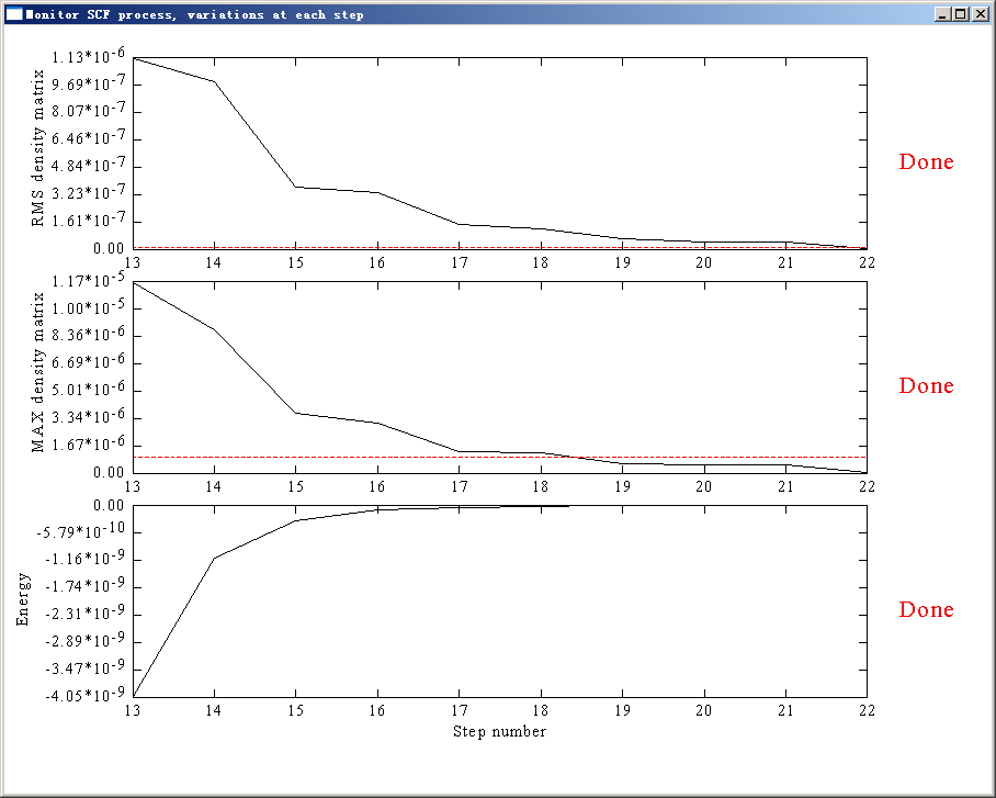
Meanwhile a window pops up, which contains curves corresponding to convergence process of energy, maximum value and RMS variation of density matrix. After you close the window, you can print the information and draw the curve graphs again in specific step range by choosing corresponding options, the Y-axis is adjusted automatically according to the data range.

If the SCF task is working in progress, that is output file is updated constantly, every time you choose to print and draw the convergence process, the Gaussian output file will be reloaded, so what you see is always the newest information. For monitoring a time-consuming SCF process, I suggest you keep the interface on until the SCF task is finished, during this period you choose option 2 every so often to show the latest 5 steps and analyze the convergence trend.

In the graph, gray dashed line shows the zero position of Y-axis, the red dashed line shows the threshold of convergence. The picture below shows the last 10 SCF steps of a system. If “Done” appears in the rightmost, that means corresponding property has already converged, here all three terms are marked by “Done”, so the entire SCF process has finished.

This function is also compatible with keyword SCF=QC and SCF=XQC, but not with SCF=DM.

3.100.8 Generate Gaussian input file with initial guess combined from fragment wavefunctions

This function is used to combine several fragment wavefunctions to an initial guess wavefunction, there are three main uses:

1 Generate high-quality initial guess wavefunction for complex

If you already have converged wavefunctions for each fragment, and the interaction between fragments is not very strong, by using the combined wavefunction as initial guess the SCF process of complex will converge faster.

2 Perform simple energy decomposition

Note

NOTE: The energy decomposition performed in the following way is strongly deprecated now! Using sobEDA or sobEDAw energy decomposition analysis (based on Multiwfn and Gaussian) is a much better choice, not only full terms can be obtained, but also much easier to use. See J. Phys. Chem. A, 127, 7023 (2023) and very detailed tutorial: http://sobereva.com/soft/sobEDA_tutorial.zip.

The total energy variation of forming a complex can be decomposed as

\[\Delta E_{\mathrm{tot}} = E^{\mathrm{complex}} - \sum_{i} E_{i}^{\mathrm{frag}} = \left( \Delta E_{\mathrm{els}} + \Delta E_{\mathrm{XC}} + \Delta E_{\mathrm{Pauli}} \right) + \Delta E_{\mathrm{orb}} = \Delta E_{\mathrm{steric}} + \Delta E_{\mathrm{orb}}\]

where Δ\(E_{\mathrm{els}}\) is electrostatic interaction term, normally negative if the fragments are neutral; Δ\(E_{\mathrm{XC}}\) is change of exchange-correlation energy during complexation process; Δ\(E_{\mathrm{Pauli}}\) comes from the Pauli repulsion effect between electrons in occupied orbitals of the fragments and is invariably positive, sometimes it is also referred to as exchange-repulsion term. For convenience, it is customary to combine these three terms as steric term (Δ\(E_{\mathrm{steric}}\)).

Δ\(E_{\mathrm{orb}}\) in above formula is orbital interaction term, it arises from the mix of occupied MOs and virtual MOs, and it exhibits polarization and charge-transfer effects. If the combined wavefunction is used as initial guess for complex, then Δ\(E_{\mathrm{orb}}\) can be evaluated by subtracting the first SCF iteration energy from the last SCF iteration energy:

\[\Delta E_{\mathrm{orb}}=E_{\mathrm{SCF,last}}-E_{\mathrm{SCF,1st}}\]

Note that \(E_{\mathrm{SCF,last}}\) = \(E^{\mathrm{complex}}\). Obviously, we have the following relationship

\[\Delta E_{\mathrm{steric}} = \Delta E_{\mathrm{tot}} - \Delta E_{\mathrm{orb}} = E_{\mathrm{SCF,1st}} - \sum_{i} E_{i}^{\mathrm{frag}}\]

By the way, if the complex you studied involves evident dispersion interaction (vdW interaction), there are two possible ways to evaluate the dispersion energy component:

• (1) Use Hartree-Fock to calculate interaction energy first (\(∆{E}_{\mathrm{tot}}^{\mathrm{HF}}\)), then use MP2 (or better post-HF method) to calculate interaction energy again (\(∆{E}_{\mathrm{tot}}^{\mathrm{MP2}}\)), then \(∆{E}_{\mathrm{disp}}=∆{E}_{\mathrm{tot}}^{\mathrm{MP2}}-∆{E}_{\mathrm{tot}}^{\mathrm{HF}}\). This relationship comes from the fact that dispersion energy is completely missing in HF energy.

• (2) Use HF or the DFT functionals that completely failed to represent dispersion energy to calculate interaction energy (e.g. B3LYP and BLYP), then use Grimme's DFT-D3 program (https://www.chemie.uni-bonn.de/grimme/de/software/dft-d3/get_dft-d3) with corresponding parameter to evaluate DFT-D3 dispersion correlation to interaction energy, which can be simply regarded as the dispersion component in total interaction energy. If you do not know how to do this and you can read Chinese, you may consult the post in my blog: http://sobereva.com/210.

An example of simple energy decomposition is given in Section 4.100.8.

3 Modelling antiferromagnetic coupling system

I will exemplify this concept and show you how to use the function by a representative antiferromagnetic coupling system -- Mn₂O₂(NH₃)₈,

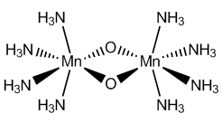
The ground state is singlet, while the two Mn atoms have opposite spin and each Mn atom has high spin. Obviously, restricted closed-shell calculation is not suitable for this system, unrestricted calculation is required, however, the default initial guess is non-symmetry-broken state, therefore the converged unrestricted wavefunction returns to restricted closed-shell wavefunction. In order to make the wavefunction converges to expected state, we have to compute wavefunction for four fragments separately and then combine them by Multiwfn to construct a proper symmetry-broken initial guess. The four fragments should be defined as

• Fragment 1: Mn(NH₃)₄ at left side. Charge = +2, sextet.

• Fragment 2: Mn(NH₃)₄ at right side. Charge = +2, sextet.

• Fragment 3: One of bridge oxygen atoms. Charge = -2, singlet.

• Fragment 4: Another bridge oxygen atom. Charge = -2, singlet.

Notice that nosymm and pop=full keywords must be specified in the calculation of each fragment. Assuming the output files are frag1.out, frag2.out, frag3.out and frag4.out, respectively, let Multiwfn load frag1.out first after booting up, then select function 100 and subfunction 8 to enter present function, input 4 to tell Multiwfn there are four fragments in total; since frag1.out has already been loaded, you only need to input the path (including filename) of frag2.out, frag3.out and frag4.out in turn. After that a Gaussian input file named new.gjf will be outputted in current directory. Notice that every time you input a fragment, Multiwfn asks you if flip its spin, only for fragment 2 you should choose y, that is make the spin direction of unpaired electrons down (by default the spin is in up direction) to exactly counteract the opposite spin in fragment 1, so that multiplicity of complex is 1.

From the comment of new.gjf (the texts behind exclamation mark), you can know clearly how the MOs of complex are combined from MOs of fragments. For example, a two-fragment system, one of complex MOs in new.gjf is

! Alpha orbital:    12 Occ:  1.000000 from fragment   2
     0.00000E+00     0.00000E+00     0.00000E+00     0.00000E+00     0.00000E+00
     0.00000E+00     0.00000E+00     0.00000E+00     0.18850E-01    -0.53690E-01
    -0.74180E-01     0.48861E+00     0.16080E+00    -0.12897E+00    -0.12897E+00
     0.47150E-01    -0.25269E+00     0.39361E+00    -0.48811E+00     0.36123E+00

We already know there are 8 basis functions in fragment 1 and 12 basis functions in fragment 2, and this complex MO comes from fragment 2, so the first 8 data (highlighted) are zero and only the last 12 data have values (the same as corresponding MO coefficients in Gaussian output file of fragment 2).

If you used diffuse functions and encounter a problem at Link401 when running new.gjf by Gaussian, you can add IOp(3/32=2) keyword and retry.

3.100.9 Evaluate interatomic connectivity and atomic coordination number

In the original paper of DFT-D3 (J. Chem. Phys., 132, 154104 (2010)), the authors argued that the coordination number (CN) of atom A can be approximately expressed as

\[CN_{A} = \sum_{B \neq A} \frac{1}{1 + \exp\{-16 \times [(4/3)(R_{A} + R_{B}) / r_{AB} - 1]\}}\]

where \(R\) is Pyykkö covalent radius from Chem. Eur. J., 15, 186 (2009), and \(r\)_AB is distance between \(A\) and \(B\).

According to this idea, in present module the interatomic connectivity index (\(I\)) between \(A\) and \(B\) is determined as follows:

\[I_{AB}(r_{AB}) = \frac{1}{1 + \exp\{-16 \times [(4/3)(R_{A} + R_{B}) / r_{AB} - 1]\}}\]

Assume that \(R\)_A+\(R\)_B=2.0, then the function could be plotted as follows. The \(I\) value equals 0.995 when \(r\)_AB=\(R\)_A+\(R\)_B

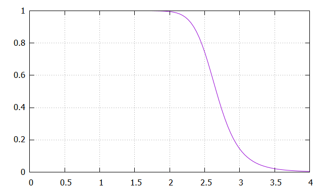
Note that the \(I\) should not be utilized as an indicator of bond order, it does not have capability of discriminating bonding type and strength.

Present module outputs \(I\) between each pair of atoms, the printing threshold can be inputted by user. Commonly, when \(I\) is close to 1.0, it implies that the two atoms are bonded, while if it is close to 0.0, then they may be regarded as not bounded by chemical bond. The nearest integer of \(I\), namely nint(\(I\)), is also outputted for facilitating examination of the result.

For each atom (e.g. atom A), the \(\sum_{B \neq A} I_{AB}\) is printed as "Sum of connectivity", while \(\sum_{B \neq A} nint(I_{AB})\) is printed as "Sum of integer connectivity". The former and the latter may be regarded as raw and actual coordination number, respectively.

Finally, you can choose if exporting all \(I\) values as matrix to connmat.txt in current folder.

Below is output example of ethyne at equilibrium geometry:

    1C   ---    2C  :   0.99951   Nearest integer:  1
    1C   ---    3H  :   0.99974   Nearest integer:  1
    2C   ---    4H  :   0.99974   Nearest integer:  1

    1  C   Sum of connectivity:  2.0016   Sum of integer connectivity:  2
    2  C   Sum of connectivity:  2.0016   Sum of integer connectivity:  2
    3  H   Sum of connectivity:  1.0021   Sum of integer connectivity:  1
    4  H   Sum of connectivity:  1.0021   Sum of integer connectivity:  1

Information needed

atom coordinates

3.100.11 Calculate overlap and centroid distance between two orbitals

This function is used to calculate overlap and centroid distance between two orbitals, this is useful for many purposes, e.g. analyzing charge transfer during electron excitation. You need to input index of two orbitals, then X, Y, Z of centroid of the orbitals will be calculated as follows

\[\begin{gathered} X_{i} = \int \left| \varphi_{i}(\mathbf{r}) \right|^{2} x \, \mathrm{d}\mathbf{r} \quad\quad Y_{i} = \int \left| \varphi_{i}(\mathbf{r}) \right|^{2} y \, \mathrm{d}\mathbf{r} \quad\quad Z_{i} = \int \left| \varphi_{i}(\mathbf{r}) \right|^{2} z \, \mathrm{d}\mathbf{r} \end{gathered}\]

then the centroid distance between orbital \(i\) and \(j\) is calculated as

\[D_{ij} = \sqrt{\left( X_{i} - X_{j} \right)^{2} + \left( Y_{i} - Y_{j} \right)^{2} + \left( Z_{i} - Z_{j} \right)^{2}}\]

Present function also calculates overlap degree of the two orbitals, below two quantities are calculated respectively (while directly calculating overlap integral of two orbital wavefunctions is clearly meaningless, since it must be zero due to orthonormalization condition):

\[\begin{gathered} \int \left| \varphi_{i}(\mathbf{r}) \right| \left| \varphi_{j}(\mathbf{r}) \right| \mathrm{d}\mathbf{r} \quad\quad \int \left| \varphi_{i}(\mathbf{r}) \right|^{2} \left| \varphi_{j}(\mathbf{r}) \right|^{2} \mathrm{d}\mathbf{r} \end{gathered}\]

The integrals shown above are not calculated analytically but numerically via Becke's grid-based integration approach. The integration grid can be set by "radpot" and "sphpot" in settings.ini, the default values are high enough, and you may want to somewhat decrease them to reduced computational cost for large system, especially when you want to study many orbital pairs.

When the calculation is finished, Multiwfn will ask you whether or not add the two centroids as two additional dummy atoms (the symbol is Bq). If you choose y, then you can go to main function 0 to visualize corresponding orbital isosurfaces by transparent or mesh style to examine correspondence between centroid position and orbital shape.

Information needed

GTFs, atom coordinates

3.100.12 Biorthogonalization between alpha and beta orbitals

Introduction

It is well known that for wavefunctions generated by unrestricted open-shell calculations (UHF or UKS), the alpha and beta orbitals are often evidently mismatch with each other, this phenomenon makes analysis of orbitals difficult, because one must simultaneously consider two set of orbitals. Although restricted open-shell (ROHF or ROKS) calculation does not have this problem, the total electronic energy, orbital energy and electron distribution is not as accurate as unrestricted open-shell calculation.

Present function is used to perform biorthogonalization between alpha and beta orbitals for unrestricted open-shell wavefunction with spin multiplicity higher than 1. Original alpha and beta molecular orbitals will be respectively transformed to a set of new orbitals. Although finally there are still two sets of orbitals, their wavefunctions have matched with each other almost perfectly, therefore then you only need to discuss one set of orbitals.

The so-called biorthogonalization mentioned here specifically refers to simultaneously satisfying two conditions: (1) For each set of spin orbitals, they are orthonormal with themselves (2) Alpha orbitals are orthonormal with respect to beta orbitals with different index. Without applying biorthogonalization, the UHF/UKS orbitals only satisfy the first condition.

Algorithm details

The biorthogonalization is realized via singular value decomposition (SVD) technique. The overlap integral matrix O between alpha and beta orbitals is first constructed, and then SVD is applied to decompose it as O=UΣV^†, where Σ is a diagonal matrix, the diagonal elements are referred to as "singular values", which essentially correspond to the overlap integrals between the orbitals after the biorthogonalization transformation, under normal situations they should be very close to 1.0. The column matrix U (V) corresponds to the transformation matrix between the original orbitals and the new orbitals of alpha (beta) spin. The coefficient matrix of the newly generated biorthogonalized orbitals can be obtained as

\[\begin{gathered} \mathbf{C}_{\mathrm{biortho}}^{\alpha} = \mathbf{U}\mathbf{C}_{\mathrm{original}}^{\alpha} \\ \mathbf{C}_{\mathrm{biortho}}^{\beta} = \mathbf{V}\mathbf{C}_{\mathrm{original}}^{\beta} \end{gathered}\]

Since U and V are unitary matrices, such a transformation does not affect observable quantities of current system.

Notice that the biorthogonalization transformation should not be done for all orbitals at once, because this will lead to mix between occupied and virtual orbitals and thus results in change of observable properties. In Multiwfn, the transformation is successively carried out via below three steps. The total number of orbitals of each spin will be denoted as \(n_{\mathrm{tot}}\), the numbers of alpha and beta electrons will be denoted as \(n\)_α and \(n\)_β, respectively. \(n\)_α>\(n\)_β is assumed.

• (1) Biorthogonalization between all occupied alpha orbitals (1~\(n\)_α) and all occupied beta orbitals (1~\(n\)_β). This step makes each resulting occupied beta orbital paired with a resulting alpha orbital.

• (2) Biorthogonalization between alpha orbitals (\(n\)_β+1~\(n\)_α) and all virtual beta orbitals (\(n\)_β+1~\(n_{\mathrm{tot}}\)). This step makes each resulting "singly occupied" alpha orbital paired with a resulting beta virtual orbital

• (3) Biorthogonalization between all alpha virtual orbitals (\(n\)_α+1~\(n_{\mathrm{tot}}\)) and the virtual beta orbitals that have not been paired (\(n\)_α+1~\(n_{\mathrm{tot}}\)).

Note

Note that in biorthogonalization steps 2 and 3, the utilized overlap integral matrix O should be reconstructed based on the coefficient matrices updated at the last step.

After these three steps of transformation, in most cases, one-to-one pairing between all alpha and beta orbitals is nicely satisfied, namely the difference between orbital wavefunction distribution of an alpha orbital and that of the beta orbital with the same index is negligible. At the same time, each alpha orbital is nearly orthogonal to a beta orbital with different index. It is noteworthy that the alpha orbitals obtained in this way are not exactly orthonormal with respect to beta orbitals, because to reach the exact orthonormalization condition, all MOs must be transformed simultaneously, which will result in undesirable mixing between occupied and unoccupied MOs.

The biorthogonalized orbitals are not eigenfunctions of Fock operator (or Kohn-Sham operator, similarly hereinafter) like molecular orbitals, however their energies can be evaluated as expectation value of Fock operator of corresponding spin. Specifically, if you request Multiwfn to evaluate the orbital energies, Multiwfn performs the following representation transformation:

\[\begin{gathered} \mathbf{F}_{\mathrm{biortho}}^{\alpha} = \left( \mathbf{C}^{\alpha} \right)^{\mathrm{T}} \mathbf{F}_{\mathrm{AO}}^{\alpha} \mathbf{C}^{\alpha} \quad\quad \mathbf{F}_{\mathrm{biortho}}^{\beta} = \left( \mathbf{C}^{\beta} \right)^{\mathrm{T}} \mathbf{F}_{\mathrm{AO}}^{\beta} \mathbf{C}^{\beta} \end{gathered}\]

where F^σ_AO is the Fock matrix of σ spin in original basis functions that loaded from external file, \(C^σ\)(µ,\(i\)) corresponds to coefficient of basis function µ in biorthogonalized orbital \(i\) of σ spin. Energy of biorthogonalized orbital \(j\) is simply \(F_{\mathrm{biortho}}\)(\(j\),\(j\)).

Note

Commonly, the numbers of α and β electrons are different, and/or their distributions are unsymmetric, therefore the single-electron effective potential (reflected by the corresponding Fock operator) of the two spins are different. So, even if you find an α and a β biorthogonalized orbitals with the same index show almost completely identical shape, their energies could be significantly different.

Once generation of orbital energies is done, Multiwfn is able to order the orbitals according to their energies. Notice that the energy used in the ordering process is average of energy of alpha orbital and its beta counterpart, and the three batch of orbitals (1~\(n\)_β), (\(n\)_β+1~\(n\)_α) and (\(n\)_α+1~\(n_{\mathrm{tot}}\)) are ordered individually (hence for example, index of an orbital originally in the second batch must still be higher than any orbital in the first batch after ordering).

Since the number of unoccupied MOs is generally much higher than the number of occupied MOs, while one often only has interest in occupied biorthogonalized orbitals, therefore Multiwfn provides an option to skip the biorthogonalization between unoccupied MOs, namely skipping the step (3) shown above. In this case the alpha and beta orbitals in the range of (\(n\)_α+1~\(n_{\mathrm{tot}}\)) will be meaningless and you should not then study them.

Usage

After booting up Multiwfn, simply loading a file containing basis function information (e.g. .mwfn, .fch, .molden, .gms) that generated by UHF or UKS calculation, then go to subfunction 12 of main function 100, you will be asked to choose if also performing biorthogonalization for unoccupied MOs, if evaluating energies of biorthogonalized orbitals, and if ordering the biorthogonalized orbitals according to their energies in the way mentioned earlier. The Fock matrix used to evaluate energies of the biorthogonalized orbitals can either be directly generated using MO energies and coefficient matrix via F=SCEC^-1, or be loaded from a file (see Appendix 7 of this manual).

After finishing the biorthogonalization, two files are exported to current folder

• biortho.txt: This file contains singular values and occupancy of the biorthogonalized orbitals. If energies of the orbitals have been evaluated, they will also be written into this file.

• biortho.fch: This file contains biorthogonalized alpha and beta orbitals. If you did not request Multiwfn to evaluate their energies, then in this file the orbital energies in a.u. will correspond to their singular values; while if their energies have been generated, then the energies will be written into this .fch file as orbital energy information.

Finally, if you input y, then the biortho.fch will be loaded directly, so that then you can directly visualize the newly generated orbitals via main function 0 or analyze them by various functions; if you input n, then the file that loaded when Multiwfn boots up will be reloaded to recover to the initial state.

Application of the biorthogonalization transformation for a practical system is illustrated in Section 4.100.12.

Information needed

Basis functions

3.100.14 Calculate LOLIPOP (LOL Integrated Pi Over Plane)

In the paper Chem. Commun., 48, 9239 (2012), the authors proposed a quantity named LOLIPOP (Localized Orbital Locator Integrated Pi Over Plane) to measure π-stacking ability of aromatic systems, they argued that a ring with smaller LOLIPOP value has stronger π-depletion (namely lower π-delocalization), and hence shows stronger π-stacking ability.

LOLIPOP is defined as definite integral of LOL-π (the LOL purely contributed by π-orbitals) from a distance of 0.5 Å away from the molecular plane. Only points with LOL-π > 0.55 are taken into account. The integration is made in a cylindrical region perpendicular to the molecular plane, with a radius of 1.94 Å corresponding to the average between the C and H ring radii in benzene.

In Multiwfn, function 14 in main function 100 is designed for calculating LOLIPOP, the default values 1.94 and 0.5 Å mentioned above can be changed by options 3 and 4 respectively. Before starting the calculation, you have to choose which orbitals are π orbitals by option 1. The calculation can be triggered by option 0, you need to input the indices of the atoms in the ring in accordance with the atom connectivity, then grid data of LOL-π around the ring will be evaluated, then the LOLIPOP value will be computed by numerical integration. Of course, smaller grid spacing gives rise to higher integration accuracy, but brings higher computational cost on evaluating LOL. The default spacing of grid data is 0.08 Bohr, this value is fine enough in general.

If you want to calculate LOLIPOP separately for each side of the ring, you can use option 5 to choose the side. By default, both sides are taken into account.

If you want to examine if the calculated LOL-π is reasonable, you can choose option 7 once, then after LOLIPOP calculation, isosurface map of LOL-π will be shown.

If you want to visually verify the distribution of the points actually included in the integration of LOLIPOP value, you can choose option 6 once, then after LOLIPOP calculation you will have pt.xyz in current folder, you can use VMD software to visualize the points recorded in this file, they correspond to the points actually contributing to LOLIPOP.

Examples of this function is provided in Section 4.100.14.

Information needed

GTFs, atom coordinates

3.100.15 Calculate intermolecular orbital overlap

This function is used to calculate orbital overlap integral between two molecules, namely

\[\begin{gathered}S_{i,j}^{\mathrm{inter}}=\int \varphi_{i}^{\mathrm{monomer1}}(\mathbf{r})\varphi_{j}^{\mathrm{monomer2}}(\mathbf{r})\mathrm{d}\mathbf{r}\end{gathered}\]

where \(i\) and \(l\) are molecular orbital indices of monomer 1 and monomer 2, respectively. This integral is useful in discussions of intermolecular charge transfer, e.g. J. Phys. Chem. B, 106, 2093 (2002).

Below three files are required for evaluating the integral, any kind of file containing basis function can be used as the input files.

• (1) Wavefunction file of dimer

• (2) Wavefunction file of monomer 1

• (3) Wavefunction file of monomer 2

To calculate the integral, after booting up Multiwfn, file (1) should be loaded first. After entering the present module, the paths of files (2) and (3) should be inputted in turn. Then you can input such as 8,15 to obtain \({S}_{8,15}^{\mathrm{inter}}\), that is the integral between MO 8 of monomer 1 and MO 15 of monomer 2. If you input letter \(o\), then the entire \(S^{\mathrm{inter}}\) matrix will be outputted to ovlpint.txt in current folder.

Notice that the atomic coordinates in files (2) and (3) must be in accordance with those in file (1), and the atomic sequence in the files should be identical. The basis set used for the three calculations must be the same. Also, notice that if in the dimer the atoms in molecule A occur prior to the atoms in molecule B, then in the present function, you must load wavefunction file of molecule A first and then load that of molecule B, otherwise the result will be incorrect.

Note

Special case:

If you are a Gaussian user, in addition to using .fch/fchk as input files, you can also use Gaussian output files for present module (though deprecated, because accuracy is slightly lower). The three files in this case should be

(1) Gaussian output file of dimer, IOp(3/33=1) nosymm guess=only should be specified in route section. Multiwfn will read overlap matrix from this file.

(2) Gaussian output file of monomer 1, nosymm pop=full should be specified in route section. Multiwfn will read orbital coefficients of monomer 1 from this file.

(3) Gaussian output file of monomer 2, nosymm pop=full should be specified in route section. Multiwfn will read orbital coefficients of monomer 2 from this file.

Corresponding example of this function is provided in Section 4.100.15.

3.100.17 Generate Fock/KS matrix based on orbital energies and coefficients

This function is used to generate one-electron effective Hamiltonian matrix based on orbital energies and expansion coefficients with respect to basis function. The generated matrix corresponds to Fock matrix for Hartree-Fock wavefunction and Kohn-Sham matrix for Kohn-Sham DFT wavefunction.

The principle of this function is very easy to comprehend: The HF or KS-DFT equation is FC=SCE, where F is Fock/KS matrix, C is coefficient matrix, S is overlap matrix, and E is a diagonal matrix whose diagonal terms correspond to various molecular orbital energies. Clearly F can be solved as F=SCEC^-1 when other matrices are available.

To use this function to yield Fock/KS matrix, after booting up Multiwfn, you should load a file containing basis function information with all molecular orbitals. For example, the .fch/.molden/.mwfn/.gms file produced by HF or DFT calculation can be used. Then enter subfunction 17 of main function 100, Fock/KS matrix will be generated in the above-mentioned way. Then you will be asked to input path of a plain text file, the generated Fock/KS matrix will be exported to it in a lower-triangular form, thus the structure of the file is:

\(F\)(1,1) \(F\)(2,1) \(F\)(2,2) \(F\)(3,1) \(F\)(3,2) \(F\)(3,3) ... \(F\)(nbasis,nbasis)

where nbasis is the total number of basis functions. For unrestricted open-shell case, alpha and beta Fock/KS matrices (Fa and Fb) are respectively generated and outputted in the following way

\(Fa\)(1,1) \(Fa\)(2,1) \(Fa\)(2,2) \(Fa\)(3,1) \(Fa\)(3,2) \(Fa\)(3,3) ... \(Fa\)(nbasis,nbasis)
\(Fb\)(1,1) \(Fb\)(2,1) \(Fb\)(2,2) \(Fb\)(3,1) \(Fb\)(3,2) \(Fb\)(3,3) ... \(Fb\)(nbasis,nbasis)

Note that some functions of Multiwfn need user to provide a file containing Fock/KS matrix so that energies of specific orbitals can be evaluated, the file exported by the present function is compatible with requirement of those functions.

It is worth to mention that due to numerical error, the Fock/KS matrix obtained as F=SCEC^-1 is inevitably lower than that originally produced by quantum chemistry code, but the difference is very small.

The present function cannot be used if linearly dependent basis functions are automatically eliminated during quantum chemistry calculation, in this case the number of solved MOs (and hence the number of loaded MO energies) is smaller than the number of basis functions. Usually this issue only occurs when diffuse functions are heavily employed.

Example

This example generates KS matrix for examples\ClPO2.fch. Boot up Multiwfn and input

examples\ClPO2.fch
100
17
ClPO2_KSmat.txt

Now you have ClPO2_KSmat.txt in current folder, which contains KS matrix elements in lower triangular form.

3.100.18 Yoshizawa's electron transport route analysis

Theory

This function is used to analyze electron transport route and is mainly based on Yoshizawa's formula (Acc. Chem. Res., 45, 1612 (2012)), At the Fermi energy, the matrix elements of the zeroth Green's function, \({G}_{rs}^{\left( 0 \right)R/A}\), which describes the propagation of a tunneling electron from site r to site s through the orbitals in a molecular part, can be written as follows:

\[G_{rs}^{(0)\mathrm{R/A}}\left( E_{\mathrm{F}} \right) = \sum_{k} \frac{C_{rk} C_{sk}^{\ast}}{E_{\mathrm{F}} - \varepsilon_{k} \pm i\eta}\]

where C_rk is the kth MO coefficient at site r, asterisk on the MO coefficient indicates a complex conjugate, ε_k is the kth MO energy, and η is an infinitesimal number determined by a relationship between the local density of states and the imaginary part of Green's function. By this formula, if two electrodes are connected to site r and s, by this formula we can readily predict the transmission probability between the two sites. From the expression of the denominator, it can be seen that HOMO and LUMO have the largest contribution to G. If only HOMO and LUMO are taken into account, the formula can be explicitly written as

\[G_{rs}^{(0)\mathrm{R/A}}\left( E_{\mathrm{F}} \right) = \frac{C_{r\mathrm{HOMO}} C_{s\mathrm{HOMO}}^{\ast}}{E_{\mathrm{F}} - \varepsilon_{\mathrm{HOMO}} \pm i\eta} + \frac{C_{r\mathrm{LUMO}} C_{s\mathrm{LUMO}}^{\ast}}{E_{\mathrm{F}} - \varepsilon_{\mathrm{LUMO}} \pm i\eta}\]

This formula allows one to visually examine the possibility of electron transmission between site r and s by means of observing molecular orbital diagram. If both site r and s have large C in magnitude, and their relative phase in HOMO and in LUMO is different, then the magnitude of G will be large, indicating that transmission between r and s will be favourable. For example, see Acc. Chem. Res., 45, 1612 (2012). Note that G may be positive and negative, but only absolute value of G is meaningful for discussing transmission.

In Multiwfn, iη term in G is always ignored, since this is an infinitesimal number. The coefficient C comes from the output of "NAOMO" keyword in NBO program. In almost all organic conductors, σ orbitals have little contribution to conductance, therefore present function only takes π orbitals into account, and the molecular plane must be parallel in XY or YZ or XZ plane.

Input file

To run this kind of analysis, there are two choices on the input file

• (1) Only using Gaussian output file

  In the route section, pop=nboread must be specified, and $NBO NAOMO $END must be written at the last line, for example:

  #P b3lyp/6-31g* pop=nboread
  
  b3lyp/6-31g* opted
  
  0 1
  [Molecular geometry field]
  
  $NBO NAOMO $END
  

• (2) Load a file containing basis function information when Multiwfn boots up, then after entering present function, load a NBO output file containing NAOMO information (namely the NAOMO keyword has been passed to NBO program. If you are using GENNBO, you can add NAOMO into $NBO…$END field of .47 file).

Usage

After you enter this function, you need to select which plane is the one your molecular plane parallel to. Then program will load file and find out the atoms having expected π atomic orbital (strictly speaking, the "Val"-type p natural atomic orbitals that perpendicular to the chosen plane). The coefficient of these atomic orbitals will be used to compute G.

Then you will see a menu, the options are explained below:

• -4 Set distance criterion: Input lower and upper limits. Then in option 2 and 3, the route whose distance exceeds this criterion will not be shown.

• -3 Set value criterion: In option 1, the MO whose contribution to G is less than this criterion will not be shown. In option 2 and 3, the route whose |G| is smaller than this criterion will not be shown.

• -2 Set Fermi energy level: Namely set \(E_{\mathrm{F}}\) in the Yoshizawa's formula.

• -1 Select the range of MOs to be considered: Namely set the MO range of the summation in the Yoshizawa's formula.

• 0 View molecular structure: As the title says.

• 1 Output detail of electron transport probability between two atoms: You need to input index for two atoms, they will be regarded as site r and s, then G_rs (the value behind "Total value") will be outputted; meanwhile program also outputs the contribution from each MO, the distance between the two atoms, and the calculated G_rs for the case when only HOMO and LUMO are taken into the summation.

• 2 Output and rank all electron transport routes in the system: All routes in current system will be tested, if the route simultaneously fulfills the G and distance criteria set by -3 and -4, then the involved atoms, G and distance of the route will be printed. The routes are ranked by absolute value of G.

• 3 Output and rank all electron transport routes for an atom: Similar to option 2, but only consider the routes involving specific atom.

Information needed

As mentioned above

3.100.19 Generate new wavefunction by combining fragment wavefunctions

This function is used to generate a new wavefunction (in .wfn., .fch or .mwfn format) by combining wavefunctions of fragments. In the new wavefunction, the electron distribution simply corresponds to the superposition of the electron distribution of the combined fragments; in other words, in this combined state the electron polarization and charge transfer between the fragments have not occurred. Each combined orbital directly corresponds to one of the fragment orbitals.

Infinite number of fragments can be combined together in this function. If .wfn file of the combined wavefunction is to be exported, the fragment wavefunction files can be in any format; however, if the wavefunction is selected to be exported as a .mwfn or .fch file, the inputted fragment wavefunctions should contain basis function information, such as .fch/mwfn/molden/gms.

Assume that the combined wavefunction consists of N fragments, after booting up Multiwfn, you should let Multiwfn load the first fragment wavefunction file, and then go to the present function (subfunction 19 of main function 100), select the format of the new wavefunction to be exported, then input the total number of fragments (N), and input the path of the wavefunction files corresponding to the other fragments in turn. Finally, you will get the wavefunction file corresponding to the combined wavefunction.

In the exported combined wavefunction file, orbitals are sorted according to orbital occupation from high to low.

If any fragment is unrestricted open-shell, then the combined wavefunction will also be unrestricted open-shell, namely the alpha and beta orbitals will separately occur in the exported wavefunction file. In this case, for each unrestricted open-shell fragment, Multiwfn will ask you if flipping the spin of its orbitals; if you input y, then the information of all alpha and all beta orbitals will be exchanged. This treatment is particularly useful if you want to get the artificial wavefunction of the whole system combined from fragment wavefunctions of free radicals.

Ghost atom may be used in fragment wavefunction calculation. If the same basis functions and atoms were employed in every fragment calculation (they only differ by the choice of ghost atoms, and union of real atoms in each fragment just corresponds to the whole system), you should input negative of number of fragments to indicate this special case. In this case only single-determinant wavefunction is supported, and only occupied orbitals will be considered to generate the combined wavefunction, while unoccupied orbitals will be ignored (if export to .fch or .mwfn format, the virtual orbitals will have zero coefficients and energies). In the combined wavefunction, all atoms will be recorded as real atoms.

An example is given in Section 4.100.19.

3.100.20 Calculate Hellmann-Feynman forces

The Hellmann-Feynman (H-F) force is the actual force acting on nuclei in a quantum system, which is exerted by electron density and other nuclei:

\[\mathbf{F}_{A} = -\left\langle \Psi \left| \frac{\partial \hat{H}}{\partial \mathbf{R}_{A}} \right| \Psi \right\rangle = \mathbf{F}_{A}^{\mathrm{ele}} + \mathbf{F}_{A}^{\mathrm{nuc}} = -Z_{A} \int \frac{\rho(\mathbf{r})\left( \mathbf{R}_{A} - \mathbf{r} \right)}{\left| \mathbf{R}_{A} - \mathbf{r} \right|^{3}} \mathrm{d}\mathbf{r} + Z_{A} \sum_{B \neq A} \frac{Z_{B}\left( \mathbf{R}_{A} - \mathbf{R}_{B} \right)}{\left| \mathbf{R}_{A} - \mathbf{R}_{B} \right|^{3}}\]

Present function calculates and prints total H-F force as well as the contribution from electron density and other nuclei respectively.

In practice, notice that the H-F forces calculated as above based on the electronic wavefunction and nuclear information recorded in the wavefunction file are generally not equivalent to the forces computed by quantum chemistry program at current calculation level (F^QC), which may be expressed as:

\[\mathbf{F}_{A}^{\mathrm{QC}} = -\frac{\partial E}{\partial \mathbf{R}_{A}} = -\left\langle \Psi \left| \frac{\partial \hat{H}}{\partial \mathbf{R}_{A}} \right| \Psi \right\rangle - 2\left\langle \partial\Psi/\partial\mathbf{R}_{A} \left| \hat{H} \right| \Psi \right\rangle\]

The partial derivative of wavefunction with respect to nuclear coordinate involves partial derivative of orbital coefficients, configuration state coefficients and basis functions with respect to R_A. Therefore, only for the fully variational wavefunctions such as HF, DFT and MCSCF with basis functions independent of nuclear coordinates (e.g. plane wave), the second term on the r.h.s. of above equation is vanishing, and then the H-F forces just equal to the force at current calculation level.

Information needed

GTFs, atom coordinates

3.100.21 Calculate properties based on geometry information for specific atoms

This function aims at characterizing structural properties of a molecule or its local region. It has many capabilities, as respectively shown below

Calculate geometry information for selected atoms

Input index range of some atoms (or input all to select the whole system), then many properties based on geometry information will be calculated for them, including

• (1) Mass

• (2) Geometry center, center of mass, center of nuclear charges

• (3) Radius of gyration

• (4) Sum of nuclear charges and dipole moments from nuclear charges

• (5) The atom having minimum/maximum coordinate in X/Y/Z

• (6) Minimum and maximum distance

• (7) Moments of inertia tensor, principal axes and principal moments of inertia

• (8) Rotational constant

• (9) Electrostatic interaction energy between nuclear charges

Note: If the input file is .chg, then "nuclear charges" mentioned above will correspond to atomic charges.

Radius of gyration is computed as

\[R_{\mathrm{g}} = \sqrt{\frac{\sum_i m_i (\mathbf{r}_i - \mathbf{r}_c)^2}{\sum_j m_j}}\]

where r is the coordinate of nucleus, r_c is mass center, m is atomic mass.

The moments of inertia tensor, which is a symmetry matrix, is calculated as

\[\mathbf{I} = \begin{bmatrix} I_{XX} & I_{XY} & I_{XZ} \\ I_{YX} & I_{YY} & I_{YZ} \\ I_{ZX} & I_{ZY} & I_{ZZ} \end{bmatrix} = \begin{bmatrix} \sum_i m_i (y_i^2 + z_i^2) & -\sum_i m_i x_i y_i & -\sum_i m_i x_i z_i \\ -\sum_i m_i y_i x_i & \sum_i m_i (x_i^2 + z_i^2) & -\sum_i m_i y_i z_i \\ -\sum_i m_i z_i x_i & -\sum_i m_i z_i y_i & \sum_i m_i (x_i^2 + y_i^2) \end{bmatrix}\]

where x, y, and z are Cartesian components of atoms relative to mass center. In the output, "The moments of inertia relative to X,Y,Z axes" correspond to the three diagonal terms of I.

The three eigenvectors of I are known as principal axes, they are outputted as the three columns of the matrix with the title "***** Principal axes (each column vector) *****". The corresponding three eigenvalues of I are the moments of inertia relative to principal axes.

If the moments of inertia are given in amu⋅Ų, then the rotational constants in GHz can be directly evaluated; for example, the rotational constant relative to Z axis is \(h/(8{\pi}^{2}{I}_{ZZ}\zeta)\mathrm{\times }{10}^{11}\), where h is Planck constant, and ξ=1.66053878*10^-27 is a factor used to convert amu to kg.

Evaluate radius, diameter, length, width and height

If you input size in this function, the system will be properly rotated to make its three principal axes respectively parallel to the three Cartesian axes. Then, according to position of boundary atoms and vdW radii proposed by Bondi (J. Phys. Chem., 68, 441 (1964)), the radius, diameter, length, width and height of present system are calculated and printed. The length, width and height can be visualized as a box enclosing the system in a GUI window, and the system can be exported as new.pdb file in current folder, which can be further visualized in VMD program.

An example is provided in Section 4.100.21.1.

Estimate distance between two fragments

If you input dist in this function, you will be asked to define two fragments, then minimum and maximum distances between the fragments, as well as distances between their geometry centers or between their mass centers, will be outputted.

Calculate area and perimeter of a ring

By inputting ring in this function, you can calculate area and perimeter of a ring. You need to input the index of the atoms in the ring in clockwise manner, for example, phenanthrene,

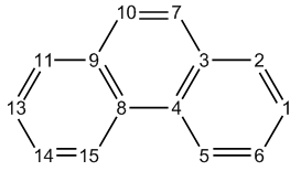
If you would like to calculate the middle ring, you should input for example 3,4,8,9,10,7.

During the calculation, the ring will be partitioned into multiple triangles, whose areas will be calculated separately and then summed up as the total area.

The ring can contain arbitrary number of atoms, and the ring may be non-planar; however, you should make sure that the ring is convex, otherwise the result could be meaningless. So, for a large ring with complex shape (e.g. porphyrin), it is better to calculate the area of its each part respectively and then manually sum them up.

It is noteworthy that in J. Org. Chem., 72, 9163 (2007), it was proposed that the aromaticity of an entire polycyclic system can be evaluated as ΣNICS(1)_ZZ/area².

Study molecular planarity

Molecular planarity has close relationship with numerous molecular properties. In J. Mol. Model., 27, 263 (2021), I proposed two rigorous, meaningful and universal metrics of planarity of a whole molecule or its local region, namely molecular planarity parameter (MPP) and span of deviation from plane (SDP), see the original paper for detail and application examples. Briefly speaking, for a given set of atoms (totally \(N_{\mathrm{atom}}\) atoms), the MPP is defined as

\[MPP = \sqrt{\frac{1}{N_{\mathrm{atom}}} \sum_i d_i^2}\]

where d_i is the distance between atom i and the plane fitted for the considered atoms.

Signed distance between atom i and the fitting plane may be expressed as

\[d_i^{\mathrm{s}} = \frac{Ax_i + By_i + Cz_i + D}{\sqrt{A^2 + B^2 + C^2}}\]

where A, B, C, D are parameters of the fitting plane. The SDP is simply defined as \({d}_{\mathrm{max}}^{\mathrm{s}}-{d}_{\mathrm{min}}^{\mathrm{s}}\), where \({d}_{\mathrm{max}}^{\mathrm{s}}\) and \({d}_{\mathrm{min}}^{\mathrm{s}}\) denote the most positive and most negative \(d^{\mathrm{s}}\) among all considered atoms, respectively.

Clearly, MPP is a straightforward measure of the overall degree of deviation of the atoms from the fitting plane, while SDP aims at exhibiting deviation span of the system with respect to the fitting plane. Obviously, the two metrics are complementary to each other.

To calculate MPP and SDP, you can input MPP after entering subfunction 21 of main function 100. Alternatively, you can directly input MPP in Multiwfn main menu. After that, you will be asked to input indices of the atoms to be considered, then the fitting plane for these atoms will be calculated, and then MPP and SDP will be outputted. Then Multiwfn can also export a .pqr file, whose “charge” property corresponds to \(d^{\mathrm{s}}\) value, hence you can use VMD software to load it and color atoms according to their “charge” properties, the relative position of the atoms with respect to the fitting plane will be vividly exhibited.

If your input file is a multiple frame .xyz file, Multiwfn will ask you to input the indices of the frames to be processed, then MPP and SDP for all selected frames will be exported to MPP_SDP.txt in current folder.

An example is provided in Section 4.100.21.2 and 4.100.21.3.

Calculate diameter of cavity

If you input cav in this function or in main menu of Multiwfn, you can enter the module for calculating diameter of cavity. I only brief describe this function here, more information is given in my blog article “Using Multiwfn to calculate cavity in molecule and crystal” http://sobereva.com/643 (in Chinese).

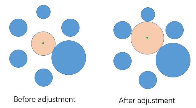
The idea behind calculation of cavity radius/diameter in Multiwfn is simple. User should first select a set of atoms that appear around the cavity and then define a sphere center (usually one can directly use the geometric center of the set of atoms), then the radius making the sphere contact nearest van der Waals (vdW) sphere of the selected atoms will be calculated, as shown by the orange sphere on the left part of the image below (green point is sphere center). In most cases, this radius cannot be used directly as the cavity radius, as it can be made larger if the center of the sphere is properly adjusted to give a more realistic picture of the actual radius of the cavity. Multiwfn iteratively adjusts the position of the sphere center by steepest ascent method to make the radius as large as possible. When the sphere center position converges (displacement less than 0.01Å), the diameter of the sphere is just the actual cavity diameter, see right part of the below figure. Note that the iteration algorithm requires that the maximum change in sphere center at each step does not exceed 0.3 Å. The vdW radii used in this function are those defined by Bondi in J. Phys. Chem., 68, 441 (1964).

Some systems contain more than one cavity. The algorithm described above can calculate any of them as long as you properly define the atoms used to detect contact and set the initial position of sphere center (during iteration process the sphere center will automatically move to the center of the nearest cavity, and thus the diameter of that cavity will be finally reported).

Examples are provided in Section 4.100.21.4.

Information needed

Atom coordinates

3.100.22 Detect π orbitals, set occupation numbers and calculate π composition

Note

It is highly encouraged to read my paper Theor. Chem. Acc., 139, 25 (2020), in which the algorithm of this module is very detailedly described and many interesting research examples are given. If this module is involved in your work, please not only cite Multiwfn original paper but also cite this paper.

This function is designed for automatically identifying π orbitals, setting occupation numbers and evaluating π composition of a given set of orbitals. This function is crucially useful for studying π electrons, e.g. calculating ELF-π. After you entered present function (subfunction 22 of main function 100), you will see an interface, you should properly select an option according to the type of your orbitals, the methods for detecting delocalized and localized orbitals are completely different.

Detecting π orbitals for delocalized orbitals

If your input file contains delocalized orbitals, e.g. molecular orbital (MO), natural orbital (NO) and natural transition orbitals (NTO), and meantime all atoms are in XY or YZ or XZ plane, you should select "0 Orbitals are in delocalized form". The program will automatically find the actual molecular plane, then during orbital detecting process, indices, occupation numbers and energies of identified π orbitals are shown on screen. After that, you can choose option 1 to set the occupation numbers of these π orbitals to zero, or choose option 2 to set the occupation number of all other orbitals to zero. Option 3 is similar to option 1, but only valence π orbitals are taken into account. Option 4 is used to clean occupation numbers for all orbitals except for valence π orbitals.

Note

For a not exactly planar system, σ and π orbitals cannot be strictly separated or defined. Sometimes, local region of a system is planar, but other atoms are not exactly in the same plane, in this case it is also possible to use present mode to detect π-like orbitals that delocalize on the local planar region. For instance, for toluene, you want to obtain index of all π-like orbitals delocalized on the six-membered ring. Before single point calculation of this system, you should make the ring exactly parallel to the XY plane, then after calculation and loading the resulting wavefunction file into Multiwfn, you should use option -4 of main function 6 to remove all GTFs on the methyl group. After that, enter present function (subfunction 2 of main function 100) and choose option 0. In this case the program will ask you to manually choose a plane because the program is unable to automatically determine the plane, you should select the option corresponding to XY plane, and then input two tolerances. Finally, three π-like orbitals will be successfully identified.

Detecting π orbitals for orbitals in localized form

If your input file contains orbitals in localized form (localized molecular orbital (LMO) is commonly employed, but others such as natural bond orbital are also supported), you should select option "-1 Orbitals are in localized form", you will enter an interface, in which if you select "0 Detect pi orbitals and then set occupation numbers", the π orbitals will be detected, and then you can set occupation number for the π orbitals or other orbitals.

The algorithm employed for this purpose was proposed by me (to be published). First, Multiwfn calculates orbital composition of present orbital and finds out the atom having largest contribution and the one having second largest contribution (they will be referred to as atoms A and B, respectively). If contribution of A is larger than a given threshold (default is 85%), then the orbital will be regarded as single-center orbital and thus be skipped. If the orbital is not singly centered, orbital density, namely |\(\varphi\)(r)|², at two probe points 0.7R_A+0.3R_B and 0.3R_A+0.7R_B, will be calculated, where R_A and R_B are coordinates of atoms A and B, respectively. If orbital density at both points is smaller than a given threshold (default is 0.01 a.u.), the orbital will be finally identified as π orbital. The idea of this identification method and the reason of introducing the density threshold is easy to understand: If an ideal π orbital forms between two atoms, since π orbital have a nodal plane along the bond, the orbital density at the two probe points on the linking line between the two atoms should be exactly zero. However, when the two atoms are not in an exactly planar local region, since σ and π orbitals are not strictly separable due to unavoidable σ-π mixing, the orbital density along the linking line must not be completely vanished, therefore a threshold is set to tolerate this circumstance.

The interface has many options. By options 1 and 2, you can set the two thresholds used in the detecting algorithm described above. By option 3, you can choose the range of orbitals for which the π ones will be identified. By option "5 Set constraint of atom range", you can set constraint of atom range by inputting atom indices. For example, if you inputted 2,4-7,9, then only the orbitals in which both the two atoms with largest contributions are in the range of 2,4,5,6,7,9 may be finally identified as π orbitals. Clearly, you can use this feature to identify all π type of LMOs lying at an interesting region, e.g. conjugated ring.

The default way of calculating the orbital compositions used for identifying the π orbitals is "Mulliken+SCPA", namely Mulliken method is used for occupied ones while SCPA method is employed for unoccupied ones, notice that in this case diffuse functions should never be used, otherwise the resulting compositions will be useless. The reason why SCPA is employed for unoccupied orbitals is that Mulliken method often gives physically meaningless compositions for them (e.g. atom with contribution larger than 100% or smaller than 0%). Via option "6 Set the method for calculating orbital composition", you can also choose other method for computing the compositions. Hirshfeld or Becke method is fully compatible with diffuse functions, they should be used if you have to employ diffuse functions when generating wavefunction. However, these two methods are relatively more expensive and according to my test, they sometimes result in wrong identification of unoccupied π orbitals (one main reason is that their results do not faithfully reflect orbital nodal character). More information about orbital composition evaluation can be found in Section 3.10.

It is worth to note that only the LMOs yielded by Pipek-Mezey orbital localization method show separation character of σ and π and thus could be used in for present function. Although Multiwfn also supports Foster-Boys localization, the σ and π characters are mixed together and result in banana type of bonds, and thus the resulting LMOs cannot be used in conjunction with present function.

Evaluating π composition for given orbitals

After selecting the "-1 Orbitals are in localized form" mentioned above, if you choose "-1 Detect pi orbitals and then evaluate pi composition for orbitals in another file", then the π type of LMOs will be detected in aforementioned way first, then you will be asked to input path of a wavefunction file, whose geometry and the number of basis functions must be exactly identical to present wavefunction.π composition of the orbitals in this file will then be evaluated based on the detected π LMOs. For example, the π composition of orbital i is evaluated as:

\[\begin{gathered} \Theta_i = 100\% \times \sum_j^{\pi\mathrm{LMO}} c_{j,i}^2 \\ c_{j,i} = \left\langle j \middle| i \right\rangle = \sum_\mu \sum_\nu C_{\mu,i} C_{\nu,j} \left\langle \chi_\mu \middle| \chi_\nu \right\rangle \end{gathered}\]

where C is orbital coefficient matrix, χ stands for basis function. You will be asked to input a threshold, only the orbitals having π composition larger than this threshold will be printed on screen.

For unrestricted wavefunction, the π compositions of alpha and beta orbitals are evaluated respectively based on alpha and beta π type of LMOs.

Note that after this analysis, the wavefunction in memory will correspond to the file you newly loaded.

There is a very important option "3 Switch the orbitals in consideration", which determines which LMOs will be employed for computing π compositions. This option has below two statuses, you need to properly choose the status according to the orbitals you want to study.

• "Occupied localized orbitals": This is default status, only occupied π LMOs will be detected and employed for evaluating π compositions. If you only want to study π compositions of occupied MOs, occupied biorthogonalized orbitals or occupied NTOs, then this status is appropriate. because it can be easily demonstrated that these orbitals are only contributed by occupied LMOs. In this case only occupied LMOs need to be obtained first.

• "All localized orbitals": All π LMOs will be detected and used for evaluating π compositions, clearly both occupied and unoccupied LMOs must be available prior to the analysis. This status can be used to evaluate π compositions for unoccupied MOs/NTOs/biorthogonalized orbitals, which are only contributed by unoccupied LMOs. If you want to evaluate π compositions for natural orbitals, you also need to switch to this status, because these orbitals can be contributed by both occupied and unoccupied LMOs.

The use of this function for orbitals in localized form is illustrated in Section 4.100.22. Sections 4.4.9 and 4.5.3 also involves this function, but for the case of delocalized orbitals.

Information needed

GTFs (delocalized orbital case), basis functions (localized orbital case), atom coordinates

3.100.23 Fit function distribution to atomic value

This function is very similar to the function used to fit ESP charge (see Section 3.9.10 and 3.9.11), but the real space function to be fitted is not limited to ESP, for example you can fit average local ionization energy or even Fukui function distributed on molecular surface to atomic values.

After selecting option 1, and then selecting a real space function, the function value will be calculated on the fitting points and then fit to atomic value by least-squares method, namely minimizing below error function

\[F(p_1, p_2 \cdots p_N) = \sum_i \left[ V(\mathbf{r}_i) - V'(\mathbf{r}_i) \right]^2\]

where i denotes the index of fitting points, p is atomic value, V is the value of real space function, while V' is the function value evaluated by atomic value, which is defined as

\[V'(\mathbf{r}_i) = \sum_A \frac{p_A}{r_{A,i}}\]

where A denotes atom index, r_A,i corresponds to the distance between nucleus of atom A and the fitting point i.

The error of fitting is measured by RMSE and RRMSE

\[\begin{gathered} \mathrm{RMSE} = \sqrt{\frac{\sum_i \left[ V(\mathbf{r}_i) - V'(\mathbf{r}_i) \right]^2}{N}} \quad\quad \mathrm{RRMSE} = \sqrt{\frac{\sum_i \left[ V(\mathbf{r}_i) - V'(\mathbf{r}_i) \right]^2}{\sum_i V(\mathbf{r}_i)^2}} \end{gathered}\]

where N denotes the number of fitting points.

By default, all fitting centers are placed at nuclei, you can also load additional fitting centers from external file by option -2, see Section 3.9.10 for the format.

The default fitting points are exactly the ones used by Merz-Kollman method (see Section 3.9.11). You can use option 3 to customize the number of layers, use option 2 to adjust the density of the fitting points distributed on the surface, and use option 4 to set the scale factor of the vdW radii used for constructing each layer. (e.g. If you set two layers, and their scale factors are set to 1.0 and 1.2 respectively, then the first and the second layer will be constructed by superposing the vdW radii of all atoms multiplied by 1.0 and 1.2, respectively)

No constraint on the total value (viz. \(\sum_{i} {p}_{i}\)) is applied by default. However, you can use option 5 to set a constraint on the total value. Evidently, if the constraint is set to the net charge of your system, and you choose ESP as fitting function, then the result will be identical to MK charges.

The fitting points can be directly defined via external plain text file by option -1 (and thus will not be constructed by superposing vdW spheres), see Section 3.9.10 for the file format. If the file contains calculated function values of all fitting points and meanwhile the first line of this file (the number of points) is set as negative value, then the real space function at each fitting point will not be evaluated by Multiwfn but loaded from this file directly.

An example of using this function to evaluate ESP fitting charge based on user-provided ESP cube file is given in #4 of http://sobereva.com/wfnbbs/viewtopic.php?pid=1542. This example illustrates the universality of this module.

Information needed

Atom coordinates