4.15 Fuzzy atomic space analysis

Introduction of basic concepts of fuzzy atomic space has been given in Section 3.18.0. In this section, a few examples will be given to illustrate some capabilities of the fuzzy atomic space analysis module. In most cases the default Becke’s definition of fuzzy atomic spaces will be employed, because it is easy to compute and reasonable for most cases. However, Hirshfeld-I and MBIS atomic spaces are more robust and evidently better in certain cases, but they need to perform iteration to refine atomic spaces, which is somewhat expensive for large systems. You can choose definition of atomic spaces used in the fuzzy analysis module by option -1.

4.15.1 Study delocalization index of benzene

The definition of delocalization index (DI) has been detailedly introduced in Section 3.18.5. DI was originally proposed for AIM atomic space, while it has been shown that if it is calculated in fuzzy atomic space, the computational cost would be significantly reduced, while the result is still meaningful. In the present instance we will calculate DI in Becke's fuzzy atomic space to study the extent of electron delocalization between different atomic pairs in benzene.

Boot up Multiwfn, and input following commands

examples\benzene.wfn  // Generated under B3LYP/6-311G*
15  // Fuzzy atomic space analysis
4  // Calculate localization index (LI) and DI. Multiwfn first makes use of DFT numerical quadrature scheme to calculate atomic overlap matrix (AOM) in each fuzzy atomic space, and then convert AOM to DI and LI.
n  // Do not output LI and DI to plain text file

Note

Multiwfn automatically checks and outputs the error of AOM, for present calculation the error is less than 0.001, which is completely negligible. If the error is too larger to be accepted, you can set "iautointgrid" in settings.ini to 0, and set "radpot" and "sphpot" to a large value. When "iautointgrid" is equal to 1, Multiwfn uses (40,230) grid points to calculate AOM, accuracy of which directly affects the accuracy of LI, DI, as well as of PDI and FLU.

From the DI matrix outputted on the screen, we can see that DI between adjacent two carbon atoms (e.g. 1-2) and adjacent C-H atoms (e.g. 1-7) are large (1.467 and 0.877, respectively), that means electron delocalization between bonded atoms is strong, this is mainly due to the shared electron of σ bond. In contrast, the DI between non-bonded carbon atoms is very small, about 0.1, nevertheless evidently not zero, reflecting the high-degree delocalization nature of π electrons.

The DI calculated in fuzzy atomic space is essentially the fuzzy bond order proposed by Mayer. According to the DI data, we can say that the bond order between C-C bond and C-H bond in benzene is 1.467 and 0.877 respectively, the former corresponds to single σ bond + "semi" π bond, while the latter corresponds to typical single σ bond.

Since benzene is an exactly planar molecule, we can decompose DI to DI-σ and DI-π. Here we calculate the latter. Input 0 to return to main menu, and then following commands

6  //Modify wavefunction
26  //Modify occupation number
0  // Select all orbitals
0  // Make occupation number of all orbitals to zero
17,20,21  // MO 17,20,21 correspond to π orbitals.
2  // Set their occupation numbers to 2 (closed-shell orbitals)
q  // Return to upper level of menu
-1  //Return to main menu

Now recalculate DI as before, since the occupation numbers of all orbitals except π orbitals have been set to zero, the result will be DI-π.

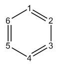
The DI-π between C1-C6, C1-C5 and C1-C4 are 0.438, 0.055 and 0.093 respectively, it is obvious that π electron delocalization is larger for para-related than for meta-related carbon atoms.

4.15.2 Study aromaticity of phenanthrene by PDI, FLU, FLU-π and PLR

PDI, FLU, FLU-π and PLR are useful aromaticity indices, their definitions have been introduced in Section 3.18.6, 3.18.7 and 3.18.9. In present instance, we will calculate them in Becke's fuzzy atomic space to study aromaticity of different rings of phenanthrene.

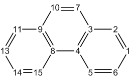
Calculate PDI

We first calculate PDI. Boot up Multiwfn, and input following commands:

examples\phenanthrene.wfn  // Optimized at B3LYP/6-31G* level
15  // Fuzzy atomic space analysis
5  // Calculate PDI

Then Multiwfn starts to calculate atomic overlap matrix (AOM), this is a computationally intensive work. After that AOM will be converted to delocalization index (DI), then DI matrix will be outputted on screen. Finally, you will be prompted to input atom indices of the ring you are interested in, the input order should be in consistent with atomic connectivity. We first calculate PDI of the central ring, namely input 4,8,9,10,7,3, the result is

Delocalization index of     4(C )   --   10(C ):    0.052992
Delocalization index of     8(C )   --    7(C ):    0.052992
Delocalization index of     9(C )   --    3(C ):    0.036334
PDI value is    0.047439

PDI value is just the average of the DIs between C4-C10, C8-C7 and C9-C3. Now we input 8,9,11,13,14,15 to calculate PDI of the boundary ring, the result is 0.0817. From this result it is evident that the electron delocalization in the boundary rings is stronger than in the central ring, so boundary rings possess larger aromaticity. Next, we use FLU and FLU-π to study the aromaticity, and check if we can draw the same conclusion.

Calculate FLU

Input q to return to upper level of menu, and input 6 to calculate FLU, then input 4,8,9,10,7,3 and 8,9,11,13,14,15 in turn. The FLU of central ring and of boundary rings are 0.025289 and 0.007499, respectively, this result suggests that the boundary rings are more likely typical aromatic systems (benzene), and hence possess larger aromaticity than the central ring. Note that since the AOM has already been calculated during calculating PDI, so this time the calculation process of AOM is automatically skipped.

Calculate FLU-π

Next, input q to return to upper level of menu, and input 7 to calculate FLU-π. First you need to input the indices of π orbitals. By visually checking isosurface of all orbitals (or utilizing option 22 in main function 100), we know that 36, 40, 43, 44, 45, 46, and 47 are π orbitals, so here we input 36,40,43,44,45,46,47, then DI of π electrons will be outputted. After that you will be prompted to input the atom indices in the ring, we input 4,8,9,10,7,3 and 8,9,11,13,14,15 in turn. The FLU-π of central ring and boundary rings are 0.149238 and 0.034904, respectively. Obviously, FLU-π analysis also confirms that boundary ring is more aromatic.

Calculate PLR

Finally, let us calculate para linear response index (PLR). PLR is based on linear response kernel, which relies on virtual MOs information; however .wfn file only contains occupied MOs, therefore we must use .mwfn/.fch/.molden/.gms file as input. Reboot Multiwfn and input following commands

examples\phenanthrene.fch  // Obtained at the same level as phenanthrene.wfn
15  // Fuzzy space analysis
10  // Calculate PLR

Multiwfn will calculate condensed linear response kernel (CLRK) matrix, after that input 4,8,9,10,7,3 and 8,9,11,13,14,15 in turn, the results are 0.248030 and 0.489560, respectively. Since the former is much smaller than the latter, PLR also validates the conclusion that boundary rings have larger aromaticity than central ring.

Note that both PDI and PLR can be separated as α and π parts to respectively investigate α and π aromaticity, see Section 3.18.6 and 3.18.9 for detail.

4.15.3 Calculate fragment dipole moment to exhibit local polarity

Note

Chinese version of this topic is my blog article “Calculation of dipole moment of molecular fragments and dipole moment of monomers in complexes using Multiwfn “ (http://sobereva.com/558, in Chinese), which contains additional example and extended discussion.

Dipole moment of a fragment may be defined as

\[\mathbf{D}_{F}=\sum_{A\in F}\left[Z_{A}\mathbf{R}_{A}-\int w_{A}(\mathbf{r})\rho(\mathbf{r})\mathbf{r}\,\mathrm{d}\mathbf{r}\right]\]

where A is atomic index in fragment F, Z_A and R_A are nuclear charge and position of atom A, respectively. w_A(r) is atomic weighting function of atom A.

As mentioned in Section 3.18.3, Multiwfn is able to calculate atomic and molecular dipole/multipole moments; if you define an atom list, then the outputted molecular dipole and multipole moments will correspond to the moments of the fragment. In this calculation, we use this feature to calculate respective dipole moment of the two monomers in phenol dimer. We will use Hirshfeld weighting function, since its calculation is easy and its physical meaning is relatively clear.

Boot up Multiwfn and input below commands

examples\phenoldimer.wfn  // Wavefunction file of optimized phenol dimer
15  // Fuzzy atomic space analysis
-1  // Select method for defining atomic space
3  // Hirshfeld based on built-in spherically averaged atomic densities
2  // Calculate atomic and molecular multipole moments
1  // Output result on screen

Then Multiwfn starts to calculate population number, dipole and multipole moments of every atom, and finally prints the data for the whole system (the "molecular" in this context corresponds to the entire current system):

              *****  Molecular dipole and multipole moments  *****
 Total number of electrons:    100.000331   Net charge: -0.000331
 Molecular dipole moment (a.u.):       1.227306     -0.128087      0.650833
 Molecular dipole moment (Debye):      3.119501     -0.325563      1.654252
 Magnitude of molecular dipole moment (a.u.&Debye):      1.395088      3.545959
 Molecular quadrupole moments (Standard Cartesian form):
 XX=  -56.973177  XY=    3.413050  XZ=    4.769915
 YX=    3.413050  YY=  -58.109370  YZ=    4.188508
 ZX=    4.769915  ZY=    4.188508  ZZ=  -57.714457
 Molecular quadrupole moments (Traceless Cartesian form):
 XX=    0.938737  XY=    5.119575  XZ=    7.154872
 YX=    5.119575  YY=   -0.765553  YZ=    6.282762
 ZX=    7.154872  ZY=    6.282762  ZZ=   -0.173184
 Magnitude of the traceless quadrupole moment tensor:    0.999096
 Molecular quadrupole moments (Spherical harmonic form):
 Q_2,0 =  -0.173184   Q_2,-1=   7.254708   Q_2,1=   8.261735
 Q_2,-2=   5.911576   Q_2,2 =   0.983972
 Magnitude: |Q_2|=   12.523257
 Molecular electronic spatial extent <r^2>:     3515.944316
 Components of <r^2>:  X=    2590.720451  Y=     631.865745  Z=     293.358120
 Molecular octopole moments (Cartesian form):
 XXX=   27.1548  YYY=  -34.6763  ZZZ=   12.9803  XYY=   31.5970  XXY=  -32.1231
 XXZ=   11.3712  XZZ=   18.8632  YZZ=   -6.4625  YYZ=   25.0005  XYZ=   21.8843
 Molecular octopole moments (Spherical harmonic form):
 Q_3,0 =   -41.5772  Q_3,-1=    25.0762  Q_3,1 =    10.2272
 Q_3,-2=    84.7574  Q_3,2 =   -26.3932  Q_3,-3=   -48.7725  Q_3,3 =   -53.4710
 Magnitude: |Q_3|=    124.8215

As can be seen, the dipole moment of the dimer is (1.227306,-0.128087,0.650833) a.u.

Next, we calculate dipole moment for the first phenol. We input

-5  // Define the atoms to be calculated
1-13  // Atom indices of the first phenol
2  // Calculate atomic and molecular multipole moments
1  // Output result on screen

You will see

Total number of electrons:     50.095624   Net charge: -0.095624
Molecular dipole moment (a.u.):       0.570356     -0.356257      0.284025
Molecular dipole moment (Debye):      1.449701     -0.905516      0.721919
Magnitude of molecular dipole moment (a.u.&Debye):      0.729997      1.855468
...[ignored]

showing that the dipole moment of the first phenol is (0.570356,-0.356257,0.284025) a.u., and the phenol carries net charge of -0.096.

Then we input

-5  // Define the atoms to be calculated
14-26  // Atom indices of the second phenol
2  // Calculate atomic and molecular multipole moments
1  // Output result on screen

You will find the second phenol has dipole moment of (0.656950 0.228171 0.366808) a.u.

In summary, now we have three dipole moments:

• dimer: (1.227306,-0.128087,0.650833) a.u.

• 1st phenol: (0.570356,-0.356257,0.284025) a.u.

• 2nd phenol: (0.656950,0.228171,0.366808) a.u.

For easily visual inspection, we will plot the dipole moments as arrows in VMD visualization program, which can be freely obtained at http://www.ks.uiuc.edu/Research/vmd/. The version I am using is VMD 1.9.3. Since VMD is unable to load .wfn file, we need to convert the present system to .xyz file. To do so, we return to main menu, enter main function 100 and choose subfunction 2, then you will find corresponding option used to export .xyz file. We export the present system as phenoldimer.xyz.

Boot up VMD and then load the phenoldimer.xyz into it. Copying all information from examples\scripts\drawarrow.tcl script file to VMD console window to run it, a new custom command "drawarrow" will be defined, which will be used to plot arrows. Then we input below commands to VMD console:

draw color green
drawarrow all 1.227306 -0.128087 0.650833 2
draw color red
drawarrow "serial 1 to 13" 0.570356 -0.356257 0.284025 2
draw color yellow
drawarrow "serial 14 to 26" 0.656950 0.228171 0.366808 2

That means dipole moment of the whole system (selected by "all") will be plotted by green arrow, that of the 1st and 2nd phenol molecules will be plotted by red and yellow arrows, respectively. The "serial 1 to 13" and "serial 14 to 26" are selection syntax in VMD. The argument "2" at the end of the commands makes the length of the arrows doubled, so that the dipole moments can be represented by the arrows clearly.

After some adjustments of graphical effect (e.g. setting drawing method as "licorice" in "Graphics" - "Representation" interface), you can see the following map. The center of the red, yellow and green arrows is placed at geometric centers of the two phenols and the dimer, respectively; the arrow lengths correspond to the norm of the dipole moments (multiplied by 2).

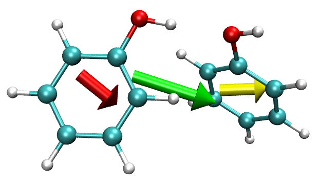
Since the dipole moment vectors of the two monomers are nearly parallel with each other, their vector sum, namely the dipole moment of the dimer, is significantly larger than the monomer dipole moments.

Bear in mind that fragment dipole moment relies on the choice of origin if the net charge of the fragment is not zero. For the present example, due to marginal charge transfer between the two phenol molecules, the monomer dipole moment must be slightly dependent of origin. However, this is not an evident problem since the net charge of the monomer is quite small and the current origin is appropriate (at nuclear charge center of the dimer).

4.15.4 Calculate atomic effective, free volumes, atomic polarizability and atomic C₆ coefficient: Oxirane and SiH₄ as examples

Note

See my blog article “Calculating atomic polarizabilities in molecules using Multiwfn” (http://sobereva.com/600, in Chinese) and “Using Multiwfn to calculate atomic C6 dispersion coefficients” (http://sobereva.com/709, in Chinese) for more discussion and examples.

Please read Section 3.18.12 first if you do not know what are atomic effective volume (\(V^{\mathrm{eff}}\)), atomic free volume (\(V^{\mathrm{free}}\)), atomic static polarizability (α^eff(0)) and atomic \(C_6\) coefficient (\(C_{6,AA}\)). In this section we will calculate them for two common molecules.

Part 1: Atomic effective/free/polarizability of oxirane

In this example we focus on evaluating \(V^{\mathrm{free}}\) and α^eff(0) for atoms in oxirane (C₂OH₄). Its wavefunction file is examples\oxirane.fchk, which was generated by Gaussian 16 at B3LYP/6-31G* level.

Prior to using Multiwfn to calculate aforementioned quantities, we need to manually generate wavefunction files of all elements (C, O, H) in the present system at the same level as molecular calculation. You can use your favourite quantum chemistry program for this step. The wavefunction files in .wfn format (H.wfn, C.wfn and O.wfn) generated by Gaussian 16 at B3LYP/6-31G* level can be directly downloaded here: http://sobereva.com/multiwfn/extrafiles/oxirane_atmvol.zip, Gaussian input files are also provided. Note that the atomic wavefunction files are not necessarily in .wfn format, they can be in any format that supported by Multiwfn, such as .mwfn, .fch and .molden.

Boot up Multiwfn and input

examples\oxirane.fchk
15  // Fuzzy analysis
13  // Calculate atomic effective volume, free volume, polarizability and \(C_6\) coefficient
H.wfn  // Path of wavefunction file of hydrogen atom in isolated state
C.wfn  // Path of wavefunction file of carbon atom in isolated state
O.wfn  // Path of wavefunction file of oxygen atom in isolated state

The output is

Atom    1(C )  Effective V:    21.536  Free V:    30.181 a.u.  Ratio: 0.714
Atom    2(C )  Effective V:    21.536  Free V:    30.181 a.u.  Ratio: 0.714
Atom    3(O )  Effective V:    21.858  Free V:    19.915 a.u.  Ratio: 1.098
Atom    4(H )  Effective V:     2.170  Free V:     6.680 a.u.  Ratio: 0.325
Atom    5(H )  Effective V:     2.170  Free V:     6.680 a.u.  Ratio: 0.325
Atom    6(H )  Effective V:     2.170  Free V:     6.680 a.u.  Ratio: 0.325
Atom    7(H )  Effective V:     2.170  Free V:     6.680 a.u.  Ratio: 0.325
Calculation took up       0 seconds wall clock time

Atomic polarizabilities estimated using Tkatchenko-Scheffler method:
   1(C ):   8.063 a.u.  Contribution: 29.01 %  (Ref. data:  11.300 a.u.)
   2(C ):   8.063 a.u.  Contribution: 29.01 %  (Ref. data:  11.300 a.u.)
   3(O ):   5.817 a.u.  Contribution: 20.92 %  (Ref. data:   5.300 a.u.)
   4(H ):   1.464 a.u.  Contribution:  5.27 %  (Ref. data:   4.507 a.u.)
   5(H ):   1.464 a.u.  Contribution:  5.27 %  (Ref. data:   4.507 a.u.)
   6(H ):   1.464 a.u.  Contribution:  5.27 %  (Ref. data:   4.507 a.u.)
   7(H ):   1.464 a.u.  Contribution:  5.27 %  (Ref. data:   4.507 a.u.)
Sum of atomic polarizabilities:    27.800 a.u.
...[ignored]

It can be seen that \(V^{\mathrm{eff}}\) of most atoms are notably reduced compared to \(V^{\mathrm{free}}\), implying that in molecular environment the polarizabilities of these atoms are decreased compared to free state, because it is well-known that there is an approximate positive correlation between volume and polarizability.

The polarizabilities of atoms in their free states (α^free(0)) are built-in data in Multiwfn and printed as “Ref. data” in above output. The atomic polarizabilities in oxirane, α^eff(0), estimated using the Tkatchenko-Scheffler method is simply product of \(V^{\mathrm{eff}}\)/\(V^{\mathrm{free}}\) and α^free(0). As shown, the sum of all α^eff(0) values is 27.8 a.u., which is in good agreement with molecular polarizability of oxirane estimated at MP2/aug-cc-pVTZ level based on current geometry (28.8 a.u.).

The sum of all α^eff(0) is not necessarily always close to molecular polarizability, and the deviation is very sensitive to the choice of atomic weighting function. For example, if you select option -1 in the fuzzy analysis interface and choose Hirshfeld partition instead of the default Becke partition, the sum of all α^eff(0) will be as high as 37.9 a.u. In this case, the “Contribution” printed by Multiwfn (α^%), which is ratio of α^eff(0) of an atom to sum of all α^eff(0), will be more useful, as its sensitivity is lower and can be used to intuitively analyze main source of molecular polarizability. For example, according to percentage atomic contribution printed by Multiwfn, we can find carbon atoms have very large contribution (each of them contributes 29% to molecular polarizability).

It is worth to mention that if interatomic interaction is extremely weak, the \(V^{\mathrm{eff}}\) should be very close to \(V^{\mathrm{free}}\). For example, \(V^{\mathrm{eff}}\) of Ar atom in Ar₂ dimer is almost identical to \(V^{\mathrm{free}}\) of Ar.

There is another way of evaluating atomic volumes in practical chemical environment, namely performing basin analysis for electron density. This idea comes from atoms-in-molecules (AIM) theory. An example can be found in Section 4.17.1.

Part 2: C₆ coefficients of SiH₄

In this example we focus on evaluating atomic \(C_6\) coefficients and homomolecular \(C_6\) coefficients in SiH₄. According to the benchmark in Section 5 of MBIS original paper (J. Chem. Theory Comput., 12, 3894 (2016)), MBIS atomic space performs best in combination with B3LYP/6-311+G(2df,p) level to evaluate molecular \(C_6\) coefficients using the Tkatchenko-Scheffler method. So, in this example we also employ this scheme. The .fch file of SiH₄ as well as .wfn file of Si and H atoms calculated at B3LYP/6-311+G(2df,p) level have been provided in “examples\SiH4_C6\” folder.

Boot up Multiwfn and input

examples\SiH4_C6\SiH4.fch
15  // Fuzzy analysis
-1  // Select the method for partitioning atomic spaces
5  // MBIS
1  // Start calculation. Then MBIS atomic spaces will be constructed
13  // Calculate atomic effective volume, free volume, polarizability and \(C_6\) coefficient
examples\SiH4_C6\H.wfn  // Wavefunction file of H atom in isolated state
examples\SiH4_C6\Si.wfn  // Wavefunction file of Si atom in isolated state

You will see the following output along with

Atomic C6 coefficients estimated using Tkatchenko-Scheffler method:
   1(Si):  118.31 a.u. (Ref. data:   305.0 a.u.)
   2(H ):    3.83 a.u. (Ref. data:     6.5 a.u.)
   3(H ):    3.83 a.u. (Ref. data:     6.5 a.u.)
   4(H ):    3.83 a.u. (Ref. data:     6.5 a.u.)
   5(H ):    3.83 a.u. (Ref. data:     6.5 a.u.)

Note: Reference data denotes the built-in value of free-state atom
Homomolecular C6 coefficient:    347.07 a.u.

You can see \(C_6\) coefficient of each atom in SiH₄. According to their magnitude, clearly the Si atom contributes to dispersion effect significantly more than H atoms. The “Ref. data” denotes \(C_6\) coefficients of atoms in their isolated state and are taken from literature. It is seen that Multiwfn also calculated and printed homomolecular \(C_6\) coefficient for SiH₄, which corresponds to the \(C_6\) coefficient used to calculate dispersion interaction between two SiH₄ molecules. The present value 347.07 a.u. is in very good agreement with the 343.9 a.u. given in Table I of J. Chem. Phys., 123, 024101 (2005)! However, it should be noted that the molecular \(C_6\) coefficient calculated in this way is not always quite accurate, sometimes the relative error may be close to 10% or even more. In addition, it should be recognized that MBIS does not perform best in all cases; for some molecules, using Hirshfeld partition may obtain better results.

4.15.5 Visualizing atomic electric dipole and quadrupole moments

Please check Section 3.18.3 to understand definition of atomic electric dipole moment (µ^A) and atomic electric quadrupole moment (Θ^A). These two quantities convey important information about electron density distribution around nuclei under a given atomic space partition scheme. In the examples in the next two sections, we will calculate and then visualize them in VMD program via a special script, you will find they are pretty intuitive and important in understanding status of atoms in actual chemical environment.

4.15.5.1 Plotting atomic dipole moments

Here I use H₂O₂ molecule as an instance to show how to calculate and plot atomic dipole moments in VMD program. VMD can be freely obtained at http://www.ks.uiuc.edu/Research/vmd/, the version I used in this example is 1.9.3.

Boot up Multiwfn and input

examples\H2O2.fch
15  // Fuzzy atomic space analysis module
2  // Calculate atomic and molecular multipole moments and
2  // Output result to a plain text file

Now you have multiple.txt and atom_moment.txt in current folder. The former contains detailed information about atomic multipole moments (from monopole moment to octopole moment), while the latter contains atomic dipole moments as well as eigenvalues and eigenvectors of atomic quadrupole moment tensors.

In order to plot atomic dipole moment vectors along with molecular structure in VMD, we need to export the geometry loaded from the H2O2.fch to H2O2.xyz by inputting the following command

0  // Return to main menu
100  // Other functions (Part 1)
2  // Export file
2  // Output current structure to .xyz file
[Press ENTER button]  // Use default file name

Now you have H2O2.xyz in current folder.

Boot up VMD, load the H2O2.xyz. Then move both atom_moment.txt and the VMD plotting script atomdip.tcl in “examples\scripts\” folder to VMD folder. Next, input the following commands in VMD console window, the first command executes the script, which defines a plotting function, while the second command runs the plotting function with default parameters.

source atomdip.tcl
atomdip

Now you can find atomic dipole moment information (in a.u.) in VMD console window:

Information of atom 1
Atomic dipole moment:  -0.198   -0.245    0.080  Norm:   0.325

 Information of atom 2
Atomic dipole moment:   0.066   -0.045   -0.043  Norm:   0.090
...[ignored]

In VMD graphical window you can see

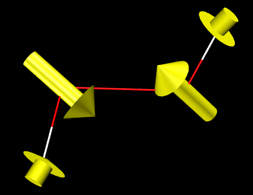
The yellow arrows correspond to µ^A vectors of every atom, pointing from negative charge center to positive charge center in corresponding atomic space, and their lengths are proportional to magnitude of µ^A. The direction of the arrow on the oxygen atoms in the figure is easy to understand. It is well known that the oxygen in H₂O₂ has obvious lone pair electrons, and the lone pair region carries a dense negative charge, while the positive charge in the atomic space is only contributed by the nuclear charge, so the arrow must approximately point from the lone pair region to the nucleus.

Adjusting graphical effects

The graphical effects can be adjusted. For example, in “Graphics” - “Representation” panel you can set drawing method as CPK and properly define thickness of bonds and radius of atom spheres. Then inputting following command in VMD console window to change background color and material of plotted objects

color Display Background white
draw material GlassBubble

Now you can see the following image

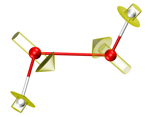
Note that the “atomdip” command has some optional parameters to control color, length, radius of arrows as well as the range of considered atoms, please check beginning of the atomdip.tcl file. As an example, if you input atomdip “serial 1 to 2 4” orange 5 0.05, arrows will be plotted only for atoms 1, 2, 4 with orange color, and the arrow length is longer than default while the arrow thickness is smaller than default.

Using different atomic space partition schemes

Dipole moment of some atoms in certain chemical environment is highly sensitive to the choice of partition of atomic spaces. You can also use other definitions of atomic spaces other than the default Becke’s definition. In fuzzy atomic space analysis module, you can use option -1 to change definition of partition.

As illustrated in Section 4.17.1, if you generate basins for electron density (i.e. AIM partition), then subfunction 8 in basin analysis module is able to calculate atomic multipole moments, and if you input y after the calculation, atom_moment.txt will be exported, based on which you can plot atomic dipole moments under AIM partition via the aforementioned procedure. You will find the direction of the arrows on oxygens in the H₂O₂ changes a lot (which, in my opinion, is not as satisfactory as Becke’s partition).

4.15.5.2 Plotting atomic quadrupole moments

In this example, we visualize atomic quadrupole moments of C₆H₅Br in VMD, the data will be calculated under Becke’s partition like the last section. The corresponding wavefunction file examples\C6H5Br.mwfn was generated at B3LYP/def-TZVP level.

Boot up Multiwfn and load examples\C6H5Br.mwfn, then use exactly the same steps as the last section to generate atom_moment.txt and C6H5Br.xyz. Move the atom_moment.txt as well as atomquad.tcl in “examples\scripts\” folder to VMD folder. Boot up VMD, load the C6H5Br.xyz, then run the following two commands in VMD console window to activate plotting script and run the plotting command

source atomquad.tcl
atomquad

After some adjustments on graphical effects, you can see

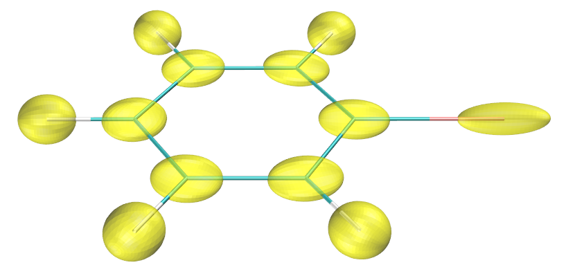
The yellow ellipsoid over each atom intuitively characterizes traceless Cartesian atomic electric quadrupole moment tensor Θ^A. The shape of the ellipsoid is determined by directions of three principal axes (eigenvectors of Θ^A) and semi-axis lengths, which are printed in VMD console window after running the “atomquad” command:

Information of atom 1
Principal axis 1:   1.000    0.000    0.000  Semi-axis length:    0.162
Principal axis 2:   0.000   -0.880    0.475  Semi-axis length:    0.405
Principal axis 3:   0.000    0.475    0.880  Semi-axis length:    0.432
...[ignored]

The ellipsoid semi-axis lengths {l} are determined via the following way proposed by me. Given that eigenvalues of Θ^A, namely {v}, may be negative, in order to make visualization feasible, they are first transformed to values equal or larger than 1 via the following equation

\[t_{i}=1+v_{i}-v_{\mathrm{min}}\qquad i=1,2,3\]

where \(v_{\mathrm{min}}\) is the most negative eigenvalue. Then {l} are evaluated as

\[l_{i}=s\frac{t_{i}}{t_{1}+t_{2}+t_{3}}\qquad i=1,2,3\]

Clearly, the sum of the three semi-axis lengths equals s, which is the scale factor controlling size of the ellipsoid, and can be set by an optional parameter of the “atomquad” command. The default value s=1 is suitable for most cases.

According to the physical meaning of Θ^A (see Section 3.18.3), it is easy to understand that the shorter the length of the ellipsoid in a certain direction, the more extended the electron density distribution in that direction, and vice versa. Therefore, from the shape of the ellipsoids in the above image, one can easily conclude that electron distribution of the carbon atoms is highly elongated in the direction perpendicular to the six-membered ring possibly due to the rich π electrons. For the Br atom, the electron density is remarkably contracted along the C-Br bond, this observation corresponds to the well-known σ-hole character.

The “atomquad” command has many optional parameters controlling the plotting effect, please check comments at beginning of the atomquad.tcl file.

In above illustration the mode 1 of the “atomquad” command was used, while by mode 2, the shape of the plotted ellipsoids can intuitively portray elongation tendency of electron density in atomic spaces. For example, by running atomquad noh green 1 2 50 in VMD console window, green ellipsoids will be drawn over all non-hydrogen atoms with scale factor of 1 and resolution of 50 using mode 2, then you can see the following figure

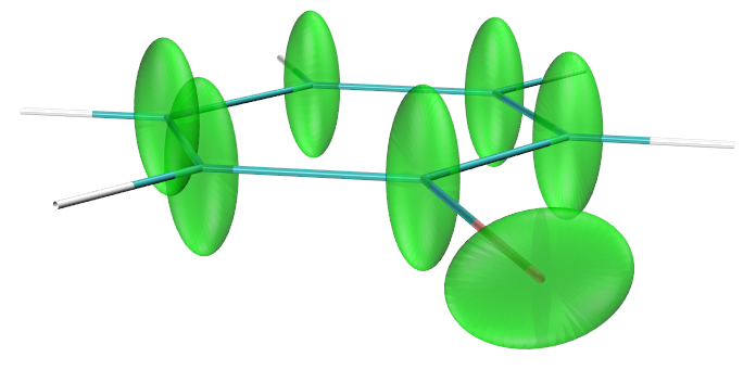
The semi-axis lengths of the ellipsoids in the map above are positively correlated to the extension extent of electron distribution in corresponding direction within atomic space. Specifically, the semi-axis lengths are evaluated in the same way as mentioned earlier but with different definition of {t}, namely

\[t_{i}=\frac{1}{1+v_{i}-v_{\mathrm{min}}}\qquad i=1,2,3\]

Above figure essentially conveys exactly the same information as the figure given earlier, but obviously this figure is more convenient for visual analysis of electron distribution. For example, it is clearly seen that in the space of Br atom, the electron density is more extended in the plane perpendicular to the C-Br bond axis.