3.19 Charge decomposition analysis and plotting orbital interaction diagram (16)

3.19.1 Theory

The charge decomposition analysis (CDA) proposed by Dapprich and Frenking (J. Phys. Chem., 99, 9352 (1995)) is used to provide deep insight into how charges are transferred between fragments in a complex to achieve charge equilibrium. The idea of CDA is based on fragment orbital (FO), which denotes the molecular orbital (MO) of fragment in its isolated state. Besides, once the compositions of FOs in MOs of complex are obtained, the orbital interaction diagram can be directly plotted, which allows one visually and directly understand how orbitals of fragments are mixed to form orbitals of complex.

For simplicity, in this section we assume that the complex consists of only two fragments. The CDA can also be straightforwardly employed for more than two fragment cases.

Fragment orbitals

Consider we are studying complex AB, NA basis functions are located in the atoms of fragment A, NB basis functions in fragment B, then each MO of complex will be linearly expanded by NA+NB basis functions, and meanwhile, the complex has NA+NB MOs. By using the same basis set, and maintaining the same geometry as in complex, if we calculate the two fragments respectively, we can obtain NA MOs of fragment A, and NB MOs of fragment B, they are collectively called fragment orbital (FO). We can take these FOs as basis functions to linearly expand the MOs of complex. Since the dimension (the number of basis functions) is still NA+NB, the expansion is exact. In other words, we equivalently transformed the basis.

Charge decomposition analysis

In the original paper of CDA, the authors defined three terms:

\[\begin{gathered}d_i=\sum_{m\in A}^{\mathrm{occ}}\sum_{n\in B}^{\mathrm{vir}}\eta_i C_{m,i}C_{n,i}S_{m,n}\\ b_i=\sum_{m\in A}^{\mathrm{vir}}\sum_{n\in B}^{\mathrm{occ}}\eta_i C_{m,i}C_{n,i}S_{m,n}\\ r_i=\sum_{m\in A}^{\mathrm{occ}}\sum_{n\in B}^{\mathrm{occ}}\eta_i C_{m,i}C_{n,i}S_{m,n}\end{gathered}\]

where i and η are index and occupation number of MO of complex, respectively. \(S_{m,n}=\int\varphi_m(\mathbf{r})\varphi_n(\mathbf{r})\mathrm{d}\mathbf{r}\) is overlap integral between FO m and FO n. Note that though the NA and NB FOs are respectively orthonormal sets, the NA set are in common not normal to the NB set, so S is not an identity matrix. \(C_{m,i}\) denotes the coefficient of FO m in MO i of complex. The superscript "vir" and "occ" mean virtual (viz. unoccupied) and occupied, respectively.

The term \(d_{i}\) denotes the amount of electron donated from fragment A to B via MO i of complex; similarly, the term \(b_{i}\) denotes the electron back donated from B to A. In fact, η_i\(C_{m,i}\)\(C_{n,i}\)\(S_{m,n}\) can be regarded as the half of overlap population between FO m and n in MO i. Hence, the difference between term d and b is that which fragment provides its electrons from its occupied FOs to virtual FOs of another fragment. The term r reveals closed-shell interaction between two occupied FOs in different fragments; positive value of \(r_{i}\) means that owing to MO i, the electrons of the two fragments are accumulated in their overlap region and shows bonding character, while negative value indicates that the electrons are depleted from the overlap region and thus reflecting electron repulsive effect. The sum of all \(r_{i}\) terms is in general negative, because overall interaction between filled orbitals are generally repulsive. r is also known as "repulsion polarization" term

Beware that although the CDA formulae given in original paper are correct, by carefully inspecting the data, I found the d, b and r terms in the examples presented in the original paper are erroneous (the data should be divided by two).

Generalization of CDA

The original definition of CDA has two drawbacks. First, it is only applicable to closed-shell cases (namely, complex and each fragment must be closed-shell) and hence unable to be used when the two fragments are bound by covalent bonding. Second, in post-HF calculations, though the MOs of complex can be replaced by natural orbitals (NOs), the FOs can only be produced by HF or DFT calculation, because occupation numbers of FOs are not explicitly considered in the original CDA formulae.

To address the limitations of the original definition, in my paper J. Adv. Phys. Chem., 4, 111-124 (2015) (http://dx.doi.org/10.12677/JAPC.2015.44013) I proposed a generalized form of CDA, which is the form used in CDA module of Multiwfn:

\[\begin{gathered}t_i=\sum_{m\in A}\sum_{n\in B}\eta_i\frac{\left|\eta_m^{\mathrm{FO}}-\eta_n^{\mathrm{FO}}\right|}{\eta_{\mathrm{ref}}}C_{m,i}C_{n,i}S_{m,n}\\ r_i=\sum_{m\in A}\sum_{n\in B}2\frac{\min(\eta_m^{\mathrm{FO}},\eta_n^{\mathrm{FO}})}{\eta_{\mathrm{ref}}}\eta_i C_{m,i}C_{n,i}S_{m,n}\end{gathered}\]

In the generalized CDA, orbitals of complex and fragments can be produced either by HF/DFT or by post-HF method, corresponding to MOs and NOs, respectively. \({\eta}_{m}^{\mathrm{FO}}\) stands for occupation number of FO m. For open-shell cases, η_ref is 1.0, CDA will be performed for alpha spin and beta spin separately; for the former, i denotes alpha orbital of complex, m and n run over all alpha FOs; for the latter, i denotes beta orbital of complex, m and n run over all beta FOs. For closed-shell cases, η_ref is 2.0, m and n run over space orbitals. min() is the function used to extract minimum from two values. During calculation of t, if the values are only accumulated for the cases \({\eta}_{m}^{\mathrm{FO}}>{\eta}_{n}^{\mathrm{FO}}\), then the resulting t is d; if only for the cases \({\eta}_{m}^{\mathrm{FO}}<{\eta}_{n}^{\mathrm{FO}}\), then t will be b.

For the situations when the original CDA is applicable, the b and d calculated by the generalized form are exactly identical to the ones obtained via original definition; while r will be exactly twice of the one produced via original definition. The reason why factor 2 is introduced into the generalized form of r is because after doing so, r has a clearer physical meaning, namely it equals overlap population (also known as Mulliken bond order) between the occupied FOs in the two fragments.

Because the CDA has been generalized, below, FO will stand for MO or NO of fragment, "complex orbital" will denote MO or NO of complex. The orbitals can either be spin-space orbital (for open-shell) or space orbital (for closed-shell).

It is clear that the d, b and r terms can be decomposed into FO pair contributions, this kind of decomposition is supported by Multiwfn and greatly facilitates analysis of the nature of FO interaction.

Composition of FO in complex orbital and orbital interaction diagram

By using the methods discussed in Section 3.10, the composition of FO in complex orbital can be calculated. In common, Mulliken method is the best choice for this purpose, the composition of FO m in complex orbital i is calculated as

\[\Theta_{m,i}=\left(C_{m,i}^2+\sum_{n\neq m}C_{m,i}C_{n,i}S_{m,n}\right)\times 100\%\]

Note that due to a well-known drawback of Mulliken method, sometimes negative contributions may occur. Since the negative values are often not large, you can simply view them as zero. In addition, sometimes contribution may be slightly larger than 100%, you can simply view it as 100%.

Using SCPA method instead of Mulliken method to compute the composition is also supported, you just need to change “iCDAcomp” in settings.ini to 2. The advantage of SCPA over Mulliken is that the composition will never exceed 100%, and it is always positive. However, if i is a high-lying virtual orbital, the calculated composition may not be very reasonable.

From Θ, we can clearly understand how each complex orbital is formed by mixing FOs of the two fragments. Furthermore, one can plot orbital interaction diagram to visually and intuitively study the relationship between complex orbitals and FOs, namely plot a bar for each complex orbital and FO according to its energy, and then check each Θ to determine how to link the bars, e.g. if the value of Θ_m,i is larger than 5%, then the two bars corresponding to FO m and complex orbital i will be linked. Consequently, from the graph we will directly know that FO m has important contribution to complex orbital i.

Extended charge decomposition analysis (ECDA)

The difference between the total number of donation and back donation electrons, that is d - b, may be regarded as the net transferred electrons. However, in J. Am. Chem. Soc., 128, 278 (2006), the authors argued that this viewpoint is not correct, because b and d terms not only represent charge transfer effect (CT), but also electron polarization effect (PL); the latter describes the adjustment of electron distribution within the fragment, which is caused by mixing virtual and occupied FOs of the same fragment during formation of the complex, and should be excluded in the calculation of the amount of net transferred electrons. In this paper they proposed extended charge decomposition analysis (ECDA) method, by which they argued that the number of net transferred electrons can be calculated more reasonably.

In ECDA viewpoint, four terms can be defined as follows

1. PL(A) + CT(A→B) = The sum of compositions of occupied FOs of fragment A in all virtual orbitals of complex, multiplied by Occ

2. PL(A) + CT(B→A) = The sum of compositions of virtual FOs of fragment A in all occupied orbitals of complex, multiplied by Occ

3. PL(B) + CT(B→A) = The sum of compositions of occupied FOs of fragment B in all virtual orbitals of complex, multiplied by Occ

4. PL(B) + CT(A→B) = The sum of compositions of virtual FOs of fragment B in all occupied orbitals of complex, multiplied by Occ

where Occ is 1.0 and 2.0 for open-shell and closed-shell cases, respectively.

After the four terms are calculated, the number of net transferred electrons from fragment A to B can be directly obtained as

CT(A→B) - CT(B→A) = [ PL(A) + CT(A→B) ] - [ PL(A) + CT(B→A) ]

The composition of complex orbitals can be calculated by various methods, leading to different ECDA results. The method used in Multiwfn is identical to the one in ECDA original paper, namely Mulliken method.

Note that ECDA can neither be applied to post-HF calculation nor the system consisting of more than two fragments. ECDA can also not be used when SCPA is employed to evaluate orbital composition.

According to the name, ECDA is as if an extension of CDA, however in my personal opinion, ECDA is irrelevant to CDA, their basic ideas are quite different, and thus the amount of net transferred electron calculated by ECDA is not comparable with the d - b produced by CDA at all. In addition, though ECDA is realized in Multiwfn, I do not think this is a useful method. The most remarkable feature of CDA is that the electron transfer can be decomposed to contribution of complex orbitals, however ECDA is incapable to do this; ECDA can only reveal how many electrons is transferred between two fragments, but this quantity actually can be obtained by a more straightforward approach, namely calculating the fragment charge by summing up all atomic charges in the fragment, and then subtracting it by the net charge of the fragment in its isolated state.

3.19.2 Input file

CDA analysis can be carried out as long as you have files containing basis function information for complex and all fragments. As described in Section 2.5, .mwfn, .fch, .gms, .molden can be used as input file in this case.

Below requirements for input files should be noticed:

(1) The method and basis set employed in the calculation of complex and fragments must be the same, otherwise the result will be meaningless. For example, assume that you are preparing input files of CDA analysis for a transition metal complex, if mixed basis set is employed for complex calculation (e.g. Lanl2TZ for metal and 6-31G* for ligands), then in the fragment calculations, Lanl2TZ must be used for the metal fragment, and 6-31G* must be used for the ligand fragment(s).

(2) The coordinate of each fragment in their wavefunction files must be exactly identical to the coordinate in the complex wavefunction file.

Note

In order to guarantee this, it is best to first optimize the complex (and meantime obtain its wavefunction file), and then directly extract coordinates of various fragments from the optimized complex geometry and then write them as individual input files of single point task (after calculating them you will obtain wavefunction files of the fragments). Clearly, the fragments should never be optimized, otherwise their coordinates will become inconsistent with the complex coordinate.

(3) The sequence of atoms in fragments and in complex must be identical, that means the actual atom sequence in the complex can be retrieved by successively combining the atoms in fragment 1, 2, 3 ...

(4) Avoid employing diffuse functions whenever possible! According to my experience, when diffusion basis functions are presented, the CDA results are often unreasonable or even completely meaningless.

"examples\CDA\COBH3_ORCA" folder contains example .molden files generated by ORCA 3.0.1 for performing CDA analysis of COBH₃ system.

Special notes for Gaussian users

For Gaussian users, the points below should be noted.

• Since Gaussian automatically puts the system in standard orientation, in order to satisfy the above requirement (2), nosymm keyword should be used in the calculation to avoid this treatment.

• If you intend to use mixed basis set, and in particular Pople type basis set is involved (such as 6-31G*), it is best to specify 5d keyword in the fragment calculations to force Gaussian to use spherical-harmonic type of basis functions for d shell.

• By default, Gaussian automatically eliminates linearly dependent basis functions, hence in some cases (usually when diffuse functions are employed), the number of basis functions is not equal to the number of orbitals, in this case CDA cannot be performed. Using IOp(3/32=2) can avoid this problem.

• If you employed post-HF for complex and fragment calculations, you need to follow the steps described at the beginning of Chapter 4 to save natural orbitals into .fch file.

Gaussian output file of single point task can also be used for CDA analysis. nosymm pop=full must be employed in all cases, and IOp(3/33=1) should also be specified in the complex calculation. Molecular geometry must be given in Cartesian coordinate. If you want to perform CDA analysis at post-HF level, do not use pop=full but use density pop=NO and density pop=NOAB for closed-shell and open-shell cases, respectively, so that coefficients of natural orbitals can be outputted.

3.19.3 Usage

After booting up Multiwfn, you should first input the path of the file of complex, and then enter the CDA module. Next, you should set the number of fragments, and then input the path of the file for each fragment in turn.

For open-shell fragments, you will be prompted to choose if flipping its electron spin. If you select "y", then orbital information of its alpha and beta orbitals will be exchanged. The reason for introduction of this step is clear: for example, we want to use CDA to decompose electron transfer between fragment CH₃ and NH₂ in CH₃NH₂; CH₃NH₂ has 9 alpha and 9 beta electrons. However, during calculation via quantum chemistry codes, both CH₃ and NH₂ will be regarded as having 5 alpha and 4 beta electrons. Therefore, in order to carry out CDA, we have to flip electron spin of either CH₃ or NH₂, otherwise the total numbers of alpha and beta electrons in the two fragments, namely 5+5=10 and 4+4=8, respectively, will be unequal to those of the complex, namely 9 and 9.

Once the loading is finished, Multiwfn starts to calculate some data. If only two fragments are defined, CDA and ECDA result will be directly shown. Then you will see a menu:

-3 Set threshold of printing CDA result in options 0 and -1: Only the complex orbitals with contribution to d or b or r term larger than the specified threshold in this option will be printed in option 0. This option is useful to screen out insignificant complex orbitals in printing CDA result.

-2 Switch output destination (for options 0 and 1): By default, the options 0 and 1 output results on screen; if you select this option once, then their results will be outputted to CDA.txt in current folder.

0 Print CDA result and ECDA result: Input the index of two fragments (not needed if there are only two fragments in total), then the CDA and ECDA analysis result between them will be outputted.

1 Print full CDA result: This option is only available when orbitals are natural orbitals (non-integer occupation numbers), and all complex orbitals will be shown. In contrast, in option 0, Multiwfn does not output CDA result for the complex orbitals lying higher than LUNO+4, because the number of such orbitals is often very large, whereas their contributions to d, b and r terms are often completely negligible due to their occupation numbers are often quite small.

2 Show fragment orbital contributions to specific complex orbital: If you input x, then the composition of complex orbital x will be outputted (for open-shell cases, the xth alpha and the xth beta complex orbital will be outputted respectively). By default only the FOs having contribution ≥1% will be shown, but this threshold can be altered by "compthresCDA" parameter in settings.ini.

If you want to obtain composition of a fragment orbital in all complex orbitals, you can input for example 1,6, which means orbital 6 of fragment 1 is selected.

3 Export coefficient matrix of complex orbitals in fragment orbital basis: The coefficient matrix corresponding to all FOs in all complex orbitals will be outputted to coFO.txt in current folder.

4 Export overlap matrix between fragment orbitals: The overlap matrix between all FOs will be outputted to ovlpint.txt in current folder.

6 Decompose complex orbital contribution to CDA: You need to input index of a complex orbital and set threshold for printing, if contribution of a pair of fragmental orbitals to any of d, b and r term of this complex orbital is larger than the threshold then the contribution value will be shown. This greatly facilitates analysis of interaction between fragment orbitals.

5 Plot orbital interaction diagram: If you select this option, you will enter a new menu, in which by corresponding options you can plot and save orbital interaction diagram and adjust plotting parameters, such as size of labels, energy range (namely Y-axis range) and the criterion for linking bars. The orbital interaction diagram plotted under default settings looks like this:

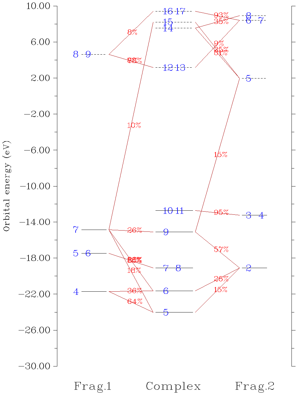
In the graph above, occupied and virtual orbitals are represented as solid and dashed bars, respectively, the vertical positions are determined by their energies. The bars at left and right sides correspond to the FOs of the two fragments you selected; the bars in the middle correspond to complex orbitals. Orbital indices are labelled by blue texts. If two or more labels occur in the same bar, that means these orbitals are degenerated in energy. If composition of a FO in a complex orbital is larger than specific criterion, then the corresponding two bars will be connected by red line, so that simply by viewing the diagram one can directly understand the complex orbitals are constructed by mainly mixing which FOs. The compositions are labelled in the center of the lines.

By default, all FOs and complex MOs are plotted, and if the contribution of a FO of fragment A or B to a complex MO is larger than 10% then they will be connected. For large systems, usually there are too many bars and linking lines in the diagram, and it is hence difficult to identify the orbital interaction mode based on the diagram. In these cases, you should properly use the option "4 Set the rule for connecting and drawing orbital bars" to manually set up the rule for connecting and plotting the orbital bars. See the prompt shown on the screen on how to use this option.

Sometimes the difference between orbital energies of the two fragments in the orbital interaction diagram is too large and thus hinders one to analyze the diagram, so you may want to equalize their energies. In this case, you can use the option "12 Set orbital energy shifting value" to set the value used to shifting orbital energies of the complex or the two fragments presented at the left and right side of the diagram; their orbital energies will be augmented by the given value.

Some notes

If complex or any fragment is an unrestricted open-shell system, then CDA will be performed separately for alpha and beta electrons.

Files containing restricted open-shell wavefunction can also be used as input file for CDA analysis, however, Multiwfn will deal with this situation in the same way as closed-shell case, therefore CDA data is completely wrong because occupancy of alpha and beta orbitals is incorrect, but orbital interaction diagram is still usable. If you want to correctly perform CDA based on restricted open-shell wavefunction to avoid explicitly distinguishing alpha and beta orbitals, you should manually convert restricted open-shell wavefunction to equivalent unrestricted open-shell wavefunction prior to the analysis, see Section 4.16. 4 for example.

Infinite number of fragments can be defined; however, if more than two fragments are defined, ECDA analysis will be unavailable.

ECDA analysis and orbital interaction diagram are not available if complex or any fragment was calculated by multiconfiguration method (e.g. MP2, double-hybrid functional), since orbital energy of natural orbitals is not undefined.

Some examples of CDA are given in Section 4.16.