4. Example of molecular crystal: Ice

In this section we plot IGMH map to show interactions between a water and all surrounding ones in an ice crystal.

The .cif file of ice in \(\text{I}_\text{h}\) form is file\ice\H2O-Ice-Ih.cif. We use main function 0 of Multiwfn to visualize it:

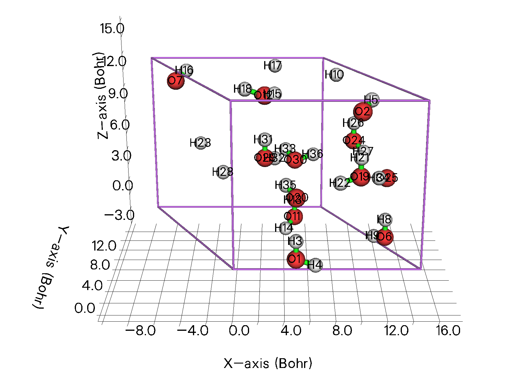
It is seen that the cell is very small (e.g. 7.36 Å in X direction). If we only consider gamma point in its periodic DFT calculation, the result would be questionable. So, we should extend it to a \(2\times 2\times 2\) supercell and then conduct calculation. Like the last example, we also need to use CP2K to optimize hydrogens.

4.1 Generate .molden file using CP2K

Boot up Multiwfn and input the following command to create CP2K input file of \(2\times 2\times 2\) supercell of ice:

H2O-Ice-Ih.cif
cp2k   // Generate CP2K input file
optH.inp   // The name of the CP2K input file to be created
-11    // Enter the interface for geometry operations
19   // Translate and duplicate cell (constructing supercell)
2   // Duplicate to twice size in the first direction
2   // Duplicate to twice size in the second direction
2   // Duplicate to twice size in the third direction
-10   // Return
-1   // Choose task
3    // Optimizing structure (cell is fixed)
9    // Set atom position constraint
optH   // Only optimize hydrogens
3    // Set dispersion correction
2   // DFT-D3(BJ)
2    // Choose basis set and pseudopotential
11    // 6-311G**
-2    // Toggle exporting .molden file for Multiwfn
0    // Generate input file now

Now we have optH.inp in current folder.

Run optH.inp by CP2K, then rename the .molden file generated last time (corresponding to the final step of geometry optimization) to optH.molden, then add the following cell information to it:

[Cell]
   15.64000000     0.00000000     0.00000000
   -7.82000000    13.54463732     0.00000000
    0.00000000     0.00000000    14.72000000

The .molden file after modification can be downloaded at http://sobereva.com/multiwfn/extrafiles/ice_supercell.rar.

4.2 Find the water at center of the supercell

Since the water at center of the supercell will be defined as a fragment of IGMH analysis, we should export the supercell structure to .pdb (or .xyz) file, so that we can then use VMD to find the water. After creating the CP2K input file of supercell (or after directly using subfunction 7 of main function 300 to construct the supercell), we input:

100    // Other functions (Part 1)
2   // Export file
1    // Output current structure to .pdb file
supercell.pdb

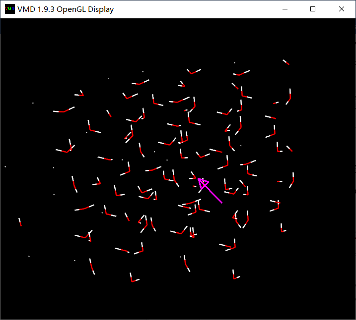
Now we have supercell.pdb in current folder. Load it to VMD, then in the graphical window, click button 0 on keyboard to enter inquire mode, then click the oxygen atom at center of the supercell, namely the atom indicated by the pink arrow below:

From console window you can see:

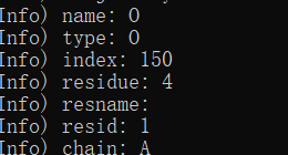
Namely this atom has index of 150 (note that "index" atomic property in VMD starts from 0 rather than 1, while the "serial" atomic property starts from 1).

Now input [atomselect top "same fragment as index 150"] get serial in VMD console window, you will see:

This information shows that the water at center of the supercell consists of atoms 10, 151, 160.

4.3 IGMH analysis in Multiwfn

Boot up Multiwfn and input:

optH.molden
20    // Visual study of weak interaction
11   // IGMH analysis
2   // Two fragments
10,151,160   // The atoms in the water at center of the supercell
c   // Set all other atoms as fragment 2
11    // Select a batch of atoms, set extension distance and grid spacing
10,151,160
3   // Extend 3 Bohr around the water at the supercell center, this is large enough
0.15   // Grid spacing of 0.15 Bohr

On my 8-core notebook, the calculation takes about 1 minute. Then export .cub files and use the IGM_inter.vmd script to plot colored \(\delta g^\text{inter}\) map in VMD as what we did in previous examples, and set isovalue of \(\delta g^\text{inter}\) to 0.03 a.u., then you can see:

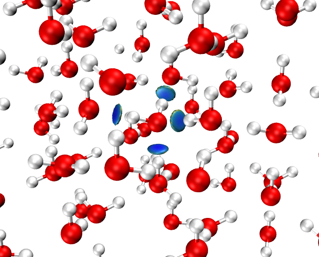
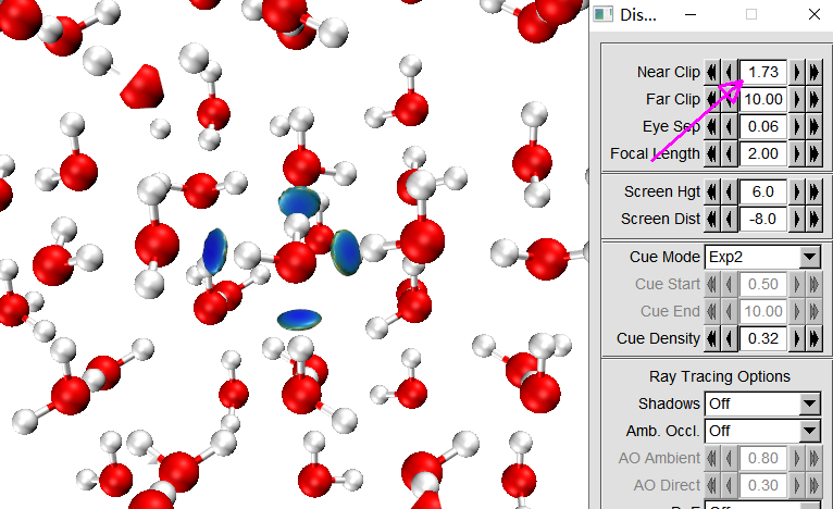
Although the H-bond interactions have been well exhibited by the blue isosurfaces, the surrounding waters evidently interfere with visual inspection of the isosurfaces. In order to improve the graphical effect, we can use "Near clip" feature to shield atoms that too close to screen.

Enter "Display" - "Display settings", properly adjust the value indicated by the arrow below until all atoms too close to screen have been shielded:

Next, we enable depth cueing to partially shield the atoms that very far from screen. Select "Display" - "Depth Cueing", then choose "Display" - "Display settings", set "Cue Mode" to "Linear", then properly adjust "Cue Start" and "Cue End":

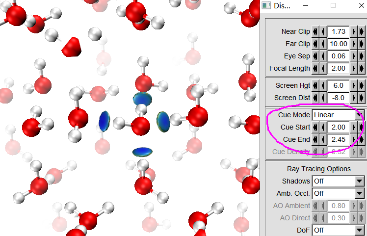
As can be seen, the graphical effect is already very good.

It is strongly advised to save the current visualization state to a file, so that next time we can immediately restore the current map. To do so, we select "File" - "Save Visualization State", browse to a proper folder and input ice.vmd. Next time, after booting up VMD, you can directly choose "File" - "Load Visualization State" and select the ice.vmd to exactly restore the above map. Note that if the dg_inter.cub and sl2r.cub files have been moved from VMD folder to another folder, or you renamed the files, you need to manually edit the ice.vmd to change the file paths (search ".cub" in this file) to actual file paths.

Hint 1

Since the water at the center of the supercell is far away from cell boundary, you can set ifdoPBCxyz in settings.ini to 0,0,0 before booting up Multiwfn. Since periodicity in all directions will then be ignored, the computational cost may be reduced notably while the result is basically not affected.

Hint 2

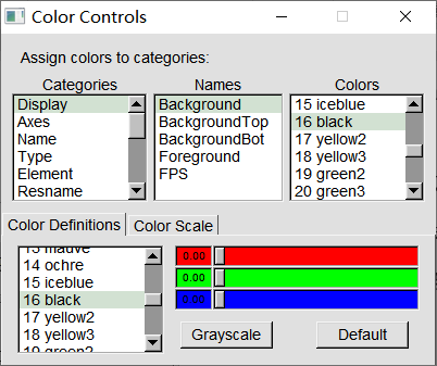
If you want to visualize box range of grid data in VMD, you should first set background to black in "Graphics" - "Colors" panel, as shown below:

Then enter "Graphics" - "Representation", choose "Box+Isosurface", see below:

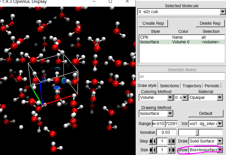
Now you can see the box range has been displayed.