3. Example of infinitely extended periodic system: Covalent organic framework (COF)

This example illustrates how to use IGMH method to reveal the interaction between the two layers in a COF cell.

.cif file of this system is file\COF\COF_12000N2.cif in this tutorial package. If you load it into Multiwfn and then enter main function 0, then choose "Other settings" - "Toggle showing cell frame" in the menu bar, you can see the following screenshot:

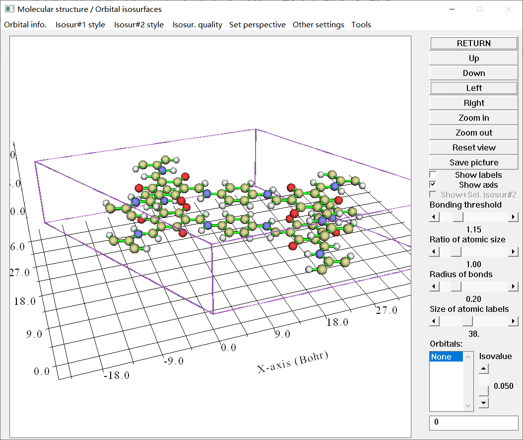
3.1 Generate CP2K input file

In order to generate the wavefunction file for IGMH analysis, we need to use CP2K first-principle program to carry out periodic DFT calculation. Since positions of hydrogens usually cannot be well determined by X-ray diffraction, we need to use CP2K to optimize hydrogens in the COF_12000N2.cif.

Input file of CP2K is known to be very difficult to manually write. Fortunately, Multiwfn has a powerful function to very easily generate input file of common tasks of CP2K. Boot up Multiwfn and input the following commands:

COF_12000N2.cif
cp2k   // Generate CP2K input file
optH.inp   // The path of the CP2K input file to be created
-1   // Choose task
3    // Optimizing structure (cell is fixed)
9    // Set atom position constraint
optH   // Only optimize hydrogens
3    // Set dispersion correction (in fact dispersion correction is not needed for present case)
2   // DFT-D3(BJ)
2    // Choose basis set and pseudopotential
11    // Use 6-311G** (for IGMH analysis in Multiwfn, 6-311G** or pob-TZVP is recommended to use, they are not expensive while the quality is satisfactory. Using the cheaper 6-31G* or def2-SVP is also acceptable. Do not use MOLOPT series of basis set, since it is fully generally contracted, if you use the resulting .molden file as input file for IGMH analysis in Multiwfn, the cost will be fairly high)
-2    // Toggle exporting .molden file for Multiwfn
0    // Generate input file now

Now you have optH.inp in current folder. It corresponds to geometry optimization only for hydrogens at PBE-D3(BJ)/6-311G** level (GAPW calculation), the size of the cell is kept fixed, and .molden file will be exported at each geometry optimization step. The current cutoff setting in this file is suitable for present system, so we will not manually change it.

It should be emphasized that CP2K does not support exporting .molden file when k-point sampling is considered, and Multiwfn also does not support consideration of k-points. So, if your cell size is small, you need to use supercell to conduct the calculation, see Section 4 for example. The current COF has a relatively large size, therefore only considering gamma point (the default case) is adequate.

3.2 Generate .molden file

Now use CP2K to run the optH.inp. Once calculation is finished, only keep the .molden file exported last time (corresponding to the finally optimized geometry) while delete all others.

We need to manually add cell information into the .molden file. Open .molden file using text editor, insert following content to line 2 of the .molden file:

[Cell]
 22.55600000     0.00000000     0.00000000
-11.27800000    19.53406901     0.00000000
  0.00000000     0.00000000     6.80000000

Each line in above content corresponds to a cell vector, which can be directly extracted from the optH.inp (note that the cell is kept unchanged during our optimization. If cell is also requested to be optimized, you can extract the cell information corresponding to the final step from output file of CP2K).

The .molden file after modification is file\COF\optH.molden, which can be directly used as input file of Multiwfn.

3.3 Performing IGMH analysis in Multiwfn

Note that if the inputted wavefunction file contains cell information (see Section 2.9 of Multiwfn manual for detail), periodic condition will be automatically enabled in IGMH analysis (and other weak interaction analyses). By default, 27 cells (1 central cell + 26 surrounding image cells) are taken into account, this is always adequate for calculating IGMH data (the number of cells taken into account can be controlled by PBCcell parameter in settings.ini, you can read Section 5.4.1 of Multiwfn manual after finishing this example!).

Boot up Multiwfn and input:

optH.molden
20    // Visual study of weak interaction
11   // IGMH analysis
2   // Two fragments
1-72   // Define the atoms in the bottom layer as fragment 1
73-144   // Define the atoms in the upper layer as fragment 2
9   // Use translation vectors of current cell, manually specify origin, box lengths and grid spacing. This mode is most suitable for the cases that isosurfaces may reach to boundary of the cell, such as the present case (evidently, the $\delta g^\text{inter}$ isosurface between the two layers must reach to cell boundary)
0,0,3   // Origin of grid data in Bohr
0,0,6   // Length of box (i.e. range of grid data) in the first, second and third cell vector directions
0.2   // Grid spacing of 0.2 Bohr.

Note that periodic IGMH analysis is much more expensive than the analysis for an isolated system with the same size. Since the present system is relatively large, you need to wait patiently. The calculation took about 6 minutes on my 8-core (Intel i7-10870H) notebook. If you feel the cost is too high, you should use a server with as many CPU cores as possible, or consider to increase grid spacing to reduce number of grid points to be calculated (of course, the smoothness of the IGMH isosurfaces will be somewhat impaired).

It is worth to explain why I inputted 0,0,3 and 0,0,6 above. The structure map with perspectives perpendicular to and parallel to the layers are respectively shown below (you can view these maps in main function 0):

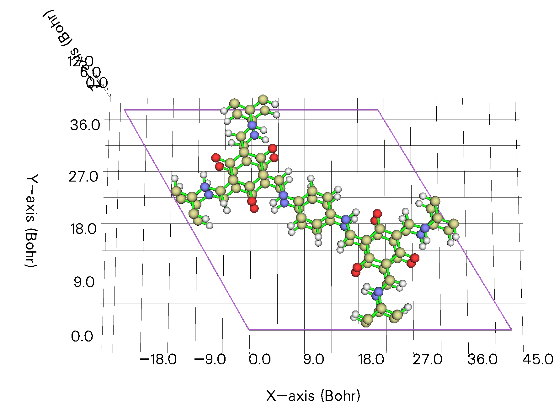
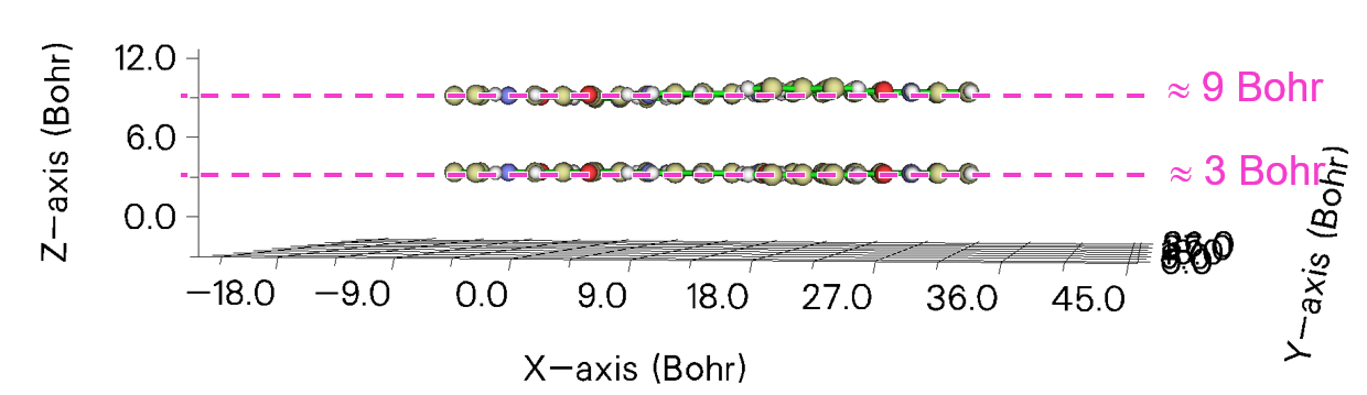
As can be seen, both X and Y coordinates of the origin of the cell are 0. The lower layer has Z coordinate of approximately 3 Bohr, therefore the origin of the grid data is suitable to be set to 0,0,3. The upper layer occurs at approximately Z = 9 Bohr, therefore the length of the grid data in the third cell direction (Z, in this context) is best to be set to \(9 - 3 = 6\) Bohr. We hope the range of grid data in the first and second cell directions to be equal to lengths of cell in corresponding directions, so we input 0,0,6 when Multiwfn asks us to set box lengths, where 0 means the length of grid data in that direction is identical to corresponding cell length.

NOTE

If you do not care about saving computational cost, or if you simply want to make grid points distributed evenly in the cell, and thus guarantee that interactions in every region will be revealed by IGMH isosurfaces, you should directly press ENTER button when Multiwfn asks you to input origin and lengths of box.

3.4 Plot IGMH map in VMD

In the post-process menu of IGMH analysis, select option -3 Output cube files to current folder to export .cub files, and then use the IGM_inter.vmd script to plot \(\delta g^\text{inter}\) map. The steps have already been carefully described in Section 1 and thus will not be repeated here. Set isovalue of \(\delta g^\text{inter}\) to 0.005, and then input pbc box in VMD console window to display border of the crystal cell, then you will see (the arrow indicates 0,0,0 position):

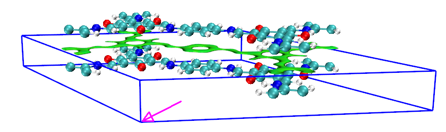
The isosurface of \(\delta g^\text{inter}\) has been correctly displayed, but the plotted cell border is evidently unreasonable. This is because the length of our grid data in the third cell direction is not identical to corresponding cell length. To solve this issue, we input the following command in VMD console window:

pbc set {22.556 22.556 6.8 90 90 120}

which sets actual length of the cell in each direction and sets actual cell angles. These data can be found when Multiwfn just finishes loading the optH.molden:

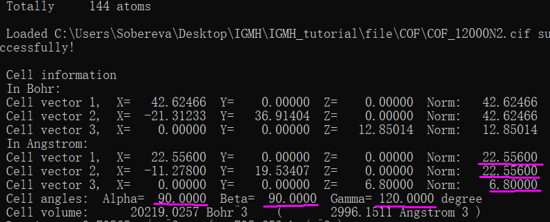
Now the IGMH map in VMD is fully reasonable:

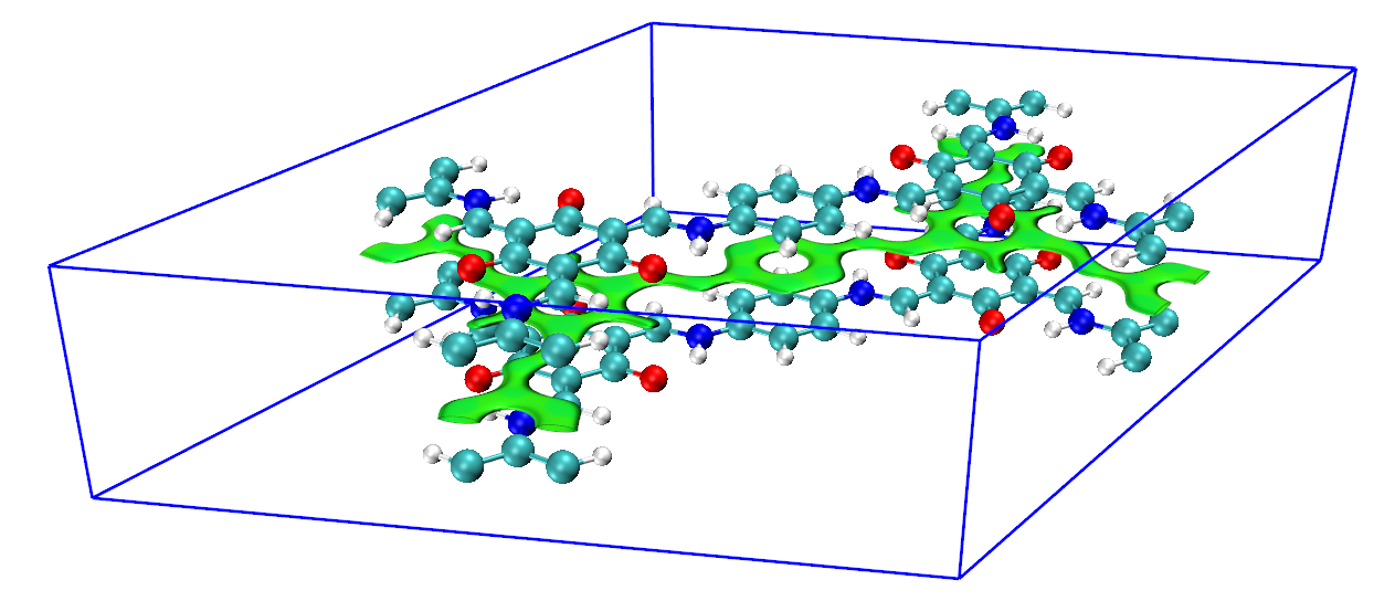
By default perspective view is used, if you want to change to orthographic view, choose "Display" - "Orthographic".

If you want to remove the blue box, input pbc box -off in VMD console window.