1. Example of a common dimer system: adenine-thymine base pair

In this example we use IGMH to analyze intermolecular in adenine-thymine base pair (AT). The optimized structure at \(\omega\)B97XD/6-311G* level is shown below. The wavefunction file in wfn format of this system is AT.wfn in the tutorial package.

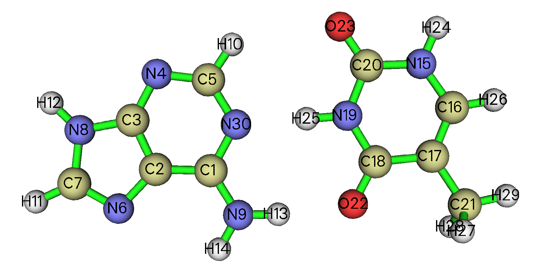
1.1 Plot \(\text{sign}(\lambda_2)\rho\) colored IGMH isosurfaces

We first plot \(\text{sign}(\lambda_2)\rho\) colored IGMH isosurface map, which is most frequently involved in IGMH analysis.

Boot up Multiwfn and input the following commands. The texts after double slash are comments:

AT.wfn  // Input actual path of input file
20  // Visual study of weak interaction
11  // IGMH analysis
2  // Define two fragments
15-29  // Indices of the atoms in the first fragment (thymine)
c  // Define the second fragment as the complement of the first fragment. So, the second fragment is the adenine
4  // Mode 4 for defining grid. You can then directly input grid spacing, the spatial range of grid data will cover the whole system. Multiwfn supports a lot of ways for defining grid, see Section 3.6 of Multiwfn manual for full description
0.15  // Using 0.15 Bohr as grid spacing.

Note that the smaller the grid spacing, the finer the isosurfaces, but the higher the computational cost and larger the resulting .cub files (the cost and file size is inversely proportional to third power of grid spacing). Usually 0.15 Bohr is sufficient to obtain a very satisfactory IGMH map, while if you want to reduce calculation cost, 0.2 Bohr is also accepted. If the grid spacing is too large, the boundary of some isosurfaces will be jaggy and ugly.

Then Multiwfn starts to calculate various grid data involved in IGMH analysis. After that, you can find the following information on screen:

Integral of delta_g over whole space:         22.930967 a.u.
Integral of delta_g_inter over whole space:    0.270387 a.u.
Integral of delta_g_intra over whole space:   22.660580 a.u.

The second line corresponds to \(\delta G^\text{inter}\) index, which is useful in quantify interfragment interaction.

Now you can see a post-process menu on screen. Multiwfn is able to directly plot isosurfaces via corresponding option. For example, to visualize \(\delta g^\text{inter}\), we should input:

4  // Show isosurface of grid data
1  // δg_inter
0.005  // Isovalue (in a.u.)

Now a GUI window appears, you can see:

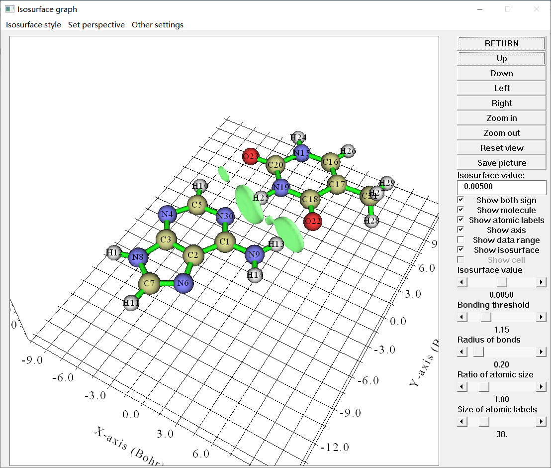
Clearly, the isosurfaces reasonably represent the expected intermolecular interactions. Then we click “RETURN” button at top right corner to close the window.

Multiwfn is unable to directly plot \(\text{sign}(\lambda_2)\rho\) colored isosurfaces, so we need to export grid data and then use VMD program to render the map. Choose option “3 Output cube files to current folder” in the post-process menu, then dg_inter.cub, dg_intra.cub, dg.cub and sl2r.cub are exported to current folder, which correspond to grid data of \(\delta g^\text{inter}\), \(\delta g^\text{intra}\), \(\delta g\) and \(\text{sign}(\lambda_2)\rho\) functions, respectively.

We move the .cub files to VMD folder, then copy VMD plotting scripts IGM_inter.vmd and IGM_intra.vmd from “examples” folder of Multiwfn package to VMD folder.

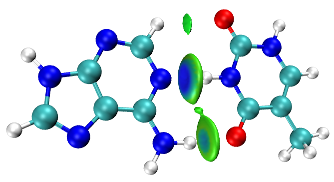
Boot up VMD, input source IGM_inter.vmd in VMD console window to execute the script, you will see \(\text{sign}(\lambda_2)\rho\) colored \(\delta g^\text{inter}\) isosurfaces:

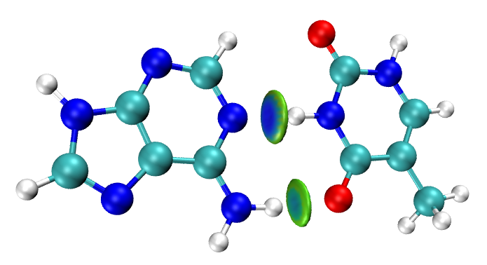
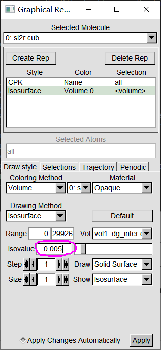
By default, the isovalue is 0.01 a.u. If you decrease it, regions corresponding to weaker interactions will also be visible. For example, we change isovalue to 0.005 a.u. To do so, select “Graphics” - “Representations”, input 0.005 in “Isovalue” box and press ENTER button:

Now you can see the map below, the region corresponds to the C-H···O interaction is also visible now:

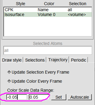
By default, the color scale range is from -0.05 to 0.05 a.u. To modify it, you can input expected values in the following box and then press ENTER button. You can also manually edit the IGM_inter.vmd script to change default color limits.

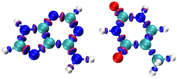
To visualize \(\text{sign}(\lambda_2)\rho\) colored \(\delta g^\text{intra}\) isosurfaces, delete the only system in VMD main window, and then input source IGM_intra.vmd in VMD console window, then you will see the following map (the default isovalue of this script is 0.2 a.u. If you increase the isovalue to 0.3 a.u., the meaningless red circle around the isosurfaces will disappear):

1.2 Evaluating \(\delta G_\text{atom}\) and \(\delta G_\text{pair}\)

To evaluate \(\delta G_\text{atom}\) and \(\delta G_\text{pair}\), in the post-process menu of IGMH we input:

6  // Evaluate contribution of atomic pairs and atoms to interfragment interaction
2  // High quality. This is good balance between accuracy and cost
y  // Export atmdg.pdb in current folder

Now in current folder you can find atmdg.txt, which contains \(\delta G_\text{atom}\) and \(\delta G_\text{atom}(\%)\) of atoms that have nonnegligible contribution to interfragment interaction, as shown below. The values are outputted from large to small:

Atom delta-g indices of fragment  1 and percentage contributions
 Atom   25 :    0.274569  (  38.21 % )
 Atom   22 :    0.146644  (  20.41 % )
 Atom   19 :    0.128561  (  17.89 % )
 Atom   18 :    0.071006  (   9.88 % )
 Atom   23 :    0.040946  (   5.70 % )
...[ignored]
 Atom delta-g indices of fragment  2 and percentage contributions
 Atom   30 :    0.228601  (  31.81 % )
 Atom   13 :    0.162840  (  22.66 % )
 Atom    9 :    0.081888  (  11.40 % )
 Atom    5 :    0.081107  (  11.29 % )
 Atom    1 :    0.073661  (  10.25 % )
...[ignored]

For example, the atom 30 in fragment 2 has \(\delta G_\text{atom}\) of 0.229 a.u. and \(\delta G_\text{atom}(\%)\) of 31.81%.

The atmdg.txt also contains \(\delta G_\text{pair}\) and \(\delta G_\text{pair}(\%)\), as shown below. The values are sorted from large to small:

Atom pair delta-g indices and percentage contributions (zero terms are not shown)
   25   30 :    0.120782  (  16.81 % )
   22   13 :    0.082451  (  11.47 % )
   19   30 :    0.057368  (   7.98 % )
   25    5 :    0.039764  (   5.53 % )
   25    1 :    0.036233  (   5.04 % )
   22    9 :    0.035627  (   4.96 % )

At the end of atmdg.txt, you can see total value:

Sum of all atom pair dg indices:    0.718566

In current folder, you can also find atmdg.pdb, it records coordinates of all atoms, and the “beta” and “occupancy” atomic properties (the data in the second-to-last and third-to-last columns) respectively correspond to \(\delta G_\text{atom}\) and \(\delta G_\text{atom}(\%)\). We can color atoms according to these indices to visually identify atoms important for interfragment interaction.

For example, here we will plot a \(\text{sign}(\lambda_2)\rho\) colored \(\delta g^\text{inter}\) isosurfaces map, and meantime color the atoms according to \(\delta G_\text{atom}(\%)\). We first use the same way as last section to plot \(\text{sign}(\lambda_2)\rho\) colored \(\delta g^\text{inter}\) isosurface map in VMD, and then drag the atmdg.pdb into VMD main window to load it. Then enter “Graphics” - “Representations” panel, and do the following steps:

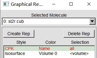
(1) Double click the representation corresponding to showing the molecular structure in the system “sl2r.cub”, then the text will become red, as shown below. Then you will find the atoms in the graphical window have disappeared:

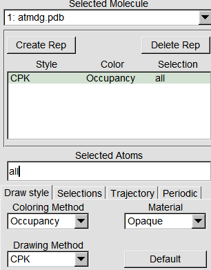
(2) Switch “Selected Molecule” to the term corresponding to “atmdg.pdb”, then set “Drawing Method” to “CPK”, set “Coloring Method” to “Occupancy”, see below:

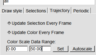
(3) Enter “Trajectory” tab, properly input upper limit of coloring. For example, we set upper limit to 50, see below, then the atom with \(\delta G_\text{atom}(\%)\) of 50 will show completely red color:

Now you can see the following map in graphical window:

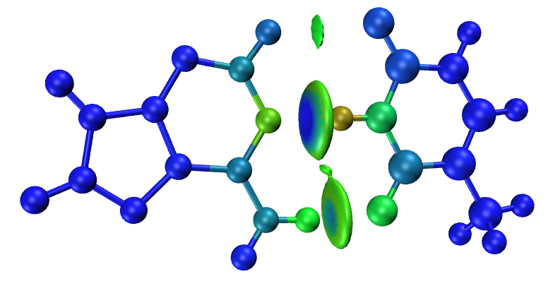
From the color you can find the atoms directly related to the two H-bonds contribute most to the interfragment interaction.

Note that the current color transition can be viewed in “Graphics” - “Colors” interface:

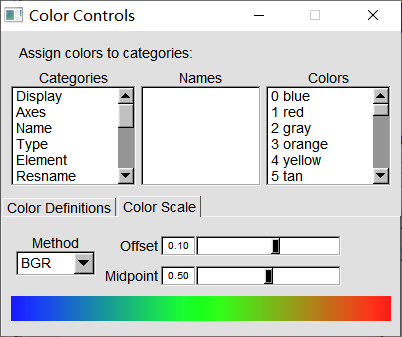
According to the color bar, it is clear that the smaller (larger) the \(\delta G_\text{atom}(\%)\) of an atom has, the bluer (redder) the color on the atom.

In addition, you can manually use e.g. PowerPoint or Photoshop software to label largest few \(\delta G_\text{pair}(\%)\) values in atmdg.txt on the IGMH map to highlight most important interatomic interactions, just like the I-AT example in the original paper of IGMH method.

1.3 Plot scatter map between \(\text{sign}(\lambda_2)\rho\) and \(\delta g\)

Scatter map between \(\text{sign}(\lambda_2)\rho\) and \(\delta g\) (or \(\delta g^\text{inter}\), \(\delta g^\text{intra}\)) is involved in some literatures employing IGM analysis, the same kind of map can also be plotted in IGMH analysis, as shown below.

In the post-process menu of IGMH analysis, select option “-1 Draw scatter graph”, then you can select corresponding suboptions to plot scatter map between \(\text{sign}(\lambda_2)\rho\) and different forms of \(\delta g\). For example, we select “4 delta_g_inter + delta_g_intra vs. sign(lambda2)rho”, then you will see:

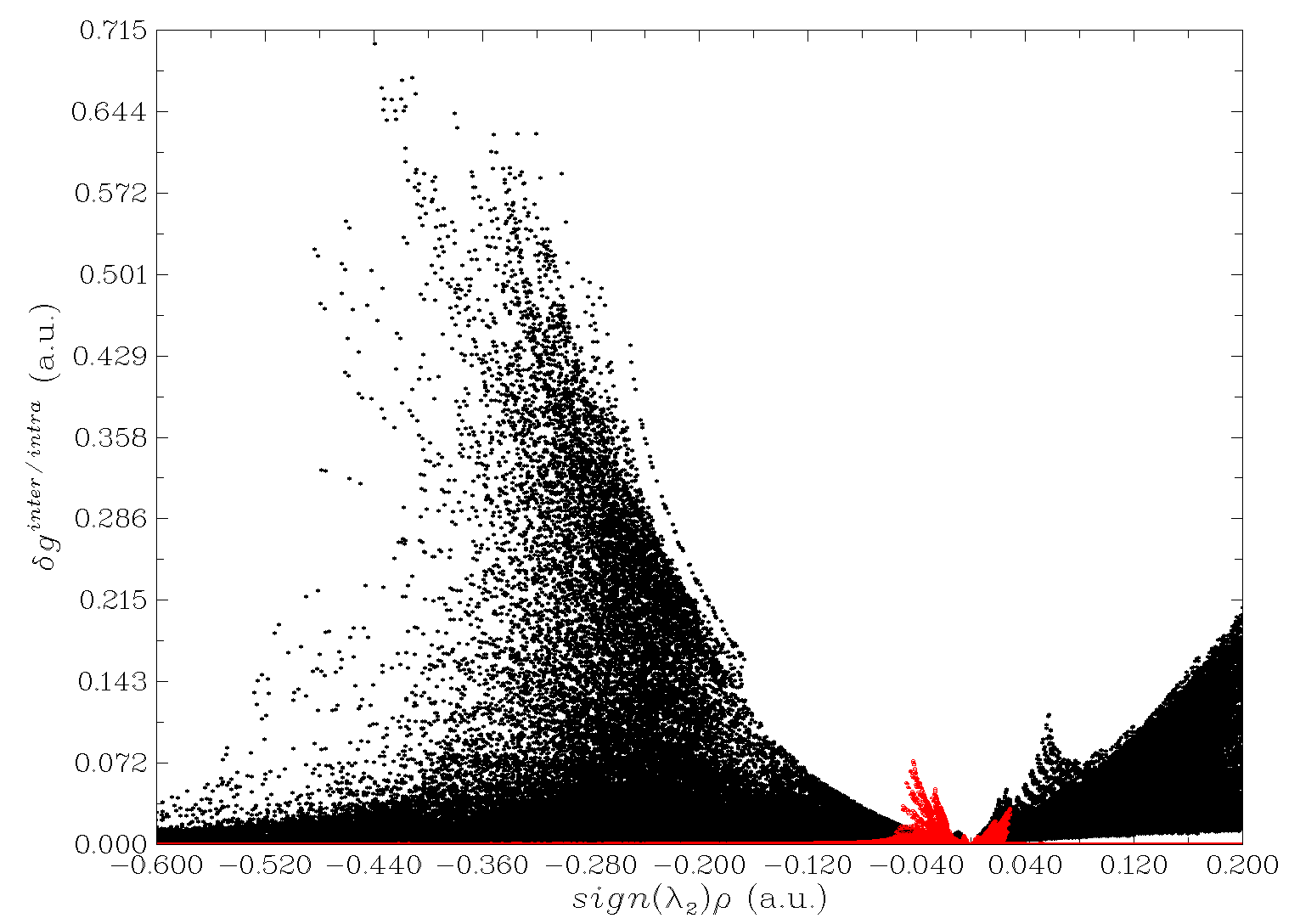
The red points correspond to “\(\text{sign}(\lambda_2)\rho\) vs. \(\delta g^\text{inter}\)” map, while the black points correspond to “\(\text{sign}(\lambda_2)\rho\) vs. \(\delta g^\text{intra}\)” map. From the position of the points, it is clear that the electron density corresponding to the intrafragment interactions is generally significantly higher than that corresponding to the interfragment interactions in this example.

You can also use my plotting script of gnuplot software (http://www.gnuplot.info) to draw \(\text{sign}(\lambda_2)\rho\) colored scatter map between \(\text{sign}(\lambda_2)\rho\) and \(\delta g^\text{inter}\), in that case you can easily identify correspondence between peaks of the scatter map and various isosurface. We select option “2 Output scatter points to output.txt in current folder” in post-process menu of IGMH analysis, the meaning of each column of the exported output.txt is shown on screen. Then copy the output.txt and the plotting script IGMscatter.gnu (in examples\scripts\ folder of Multiwfn package) to the file containing gnuplot executable file, then enter command-line interface of your system and input command .\gnuplot.exe IGMscatter.gnu, then gnuplot will run the script. After that you will obtain IGMscatter.ps in current folder. If you open it by Acrobat or Photoshop or IrfanView (with ghostscript installed), you will see the following colored scatter map. For clarity, the correspondence between the peaks and maxima of \(\delta g^\text{inter}\) in the isosurface map is indicated via arrows. This map also shows that an interaction region with larger \(\rho\) usually has larger maximum of \(\delta g^\text{inter}\) in that region.

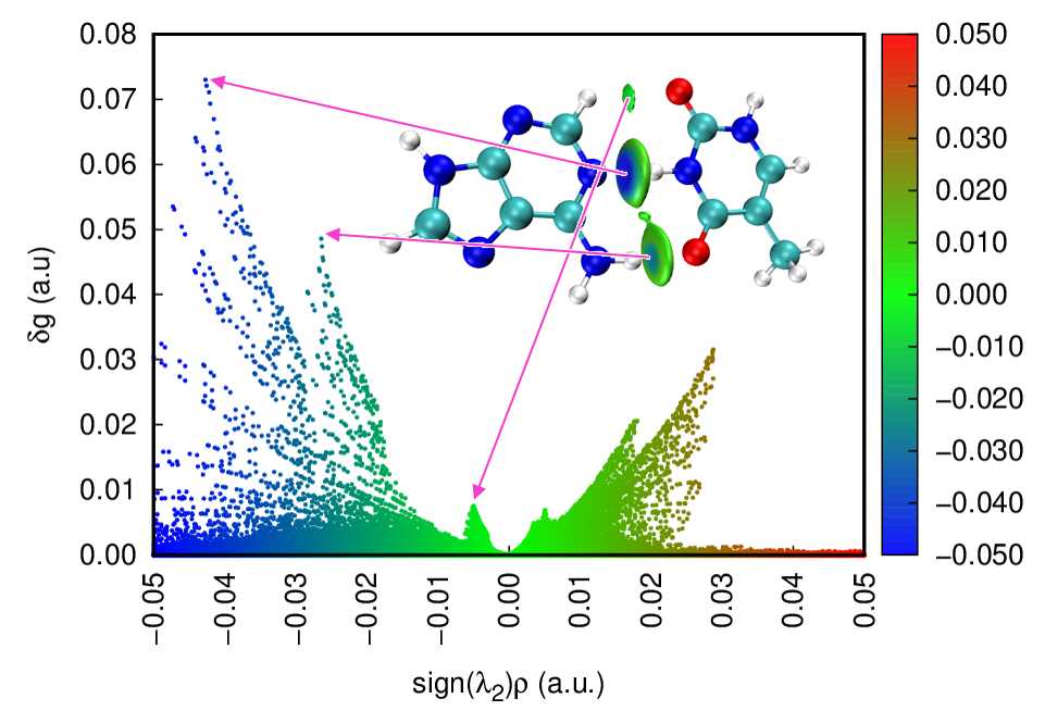
Note that the \(\delta g\) symbol on the Y-axis in the above map should be \(\delta g^\text{inter}\), you can manually edit the map or modify the plotting script.

1.4 Evaluating \(\delta g\) at bond critical points

\(\delta g\) value at bond critical point (BCP) will be referred to as \(\delta g(\text{BCP})\), this term corresponding to an interested interaction may be useful in quantifying the interaction strength. Here I illustrate how to obtain \(\delta g(\text{BCP})\) for the two H-bonds of AT. Note that very detailed examples of performing AIM topology analysis are given in Section 4.2 of Multiwfn manual.

Boot up Multiwfn and input:

AT.wfn
2  // Topology analysis
2  // Search critical points (CPs) from nuclear positions
3  // Search CPs from midpoint of atom pairs
0  // Visually inspect located CPs

In the GUI window, select “CP labels” check box at right side of the window, then you will see:

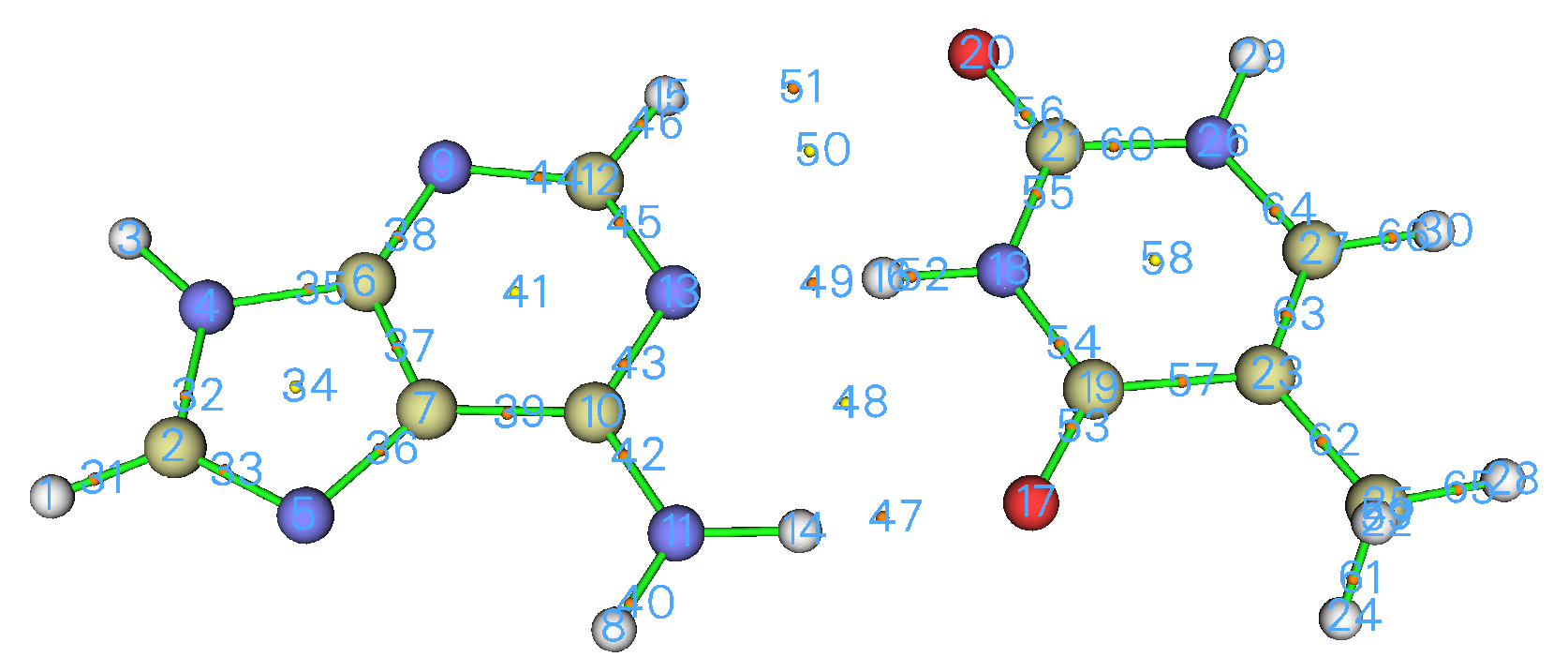
It is clear that the CP 49 and CP 47 are BCP, they correspond to N...H-N and N-H...O H-bonds, respectively. Now we evaluate \(\delta g(\text{BCP})\) for the former. Close the GUI window, then select option “7 Show real space function values at specific CP or all CPs”, and then input 49, you will see various properties at this CP:

[ignored...]
Sign(lambda2)*rho: -0.4246776763E-01
 Sign(lambda2)*rho with promolecular approximation: -0.5146725802E-01
 Corr. hole for alpha, ref.:   0.00000   0.00000   0.00000 : -0.1709500951E-01
 Source function, ref.:   0.00000   0.00000   0.00000 : -0.1060387613E-01
 Wavefunction value for orbital         1 :  0.9913266025E-05
 Average local ionization energy (ALIE):  0.5548916672E+00
 Delta_g (under promolecular approximation):  0.6696790540E-01
 Delta_g (under Hirshfeld partition):  0.7724798057E-01
 User-defined real space function:  0.1000000000E+01
 ESP from nuclear charges:  0.2524253121E+02
 ESP from electrons: -0.2506351516E+02
 Total ESP:  0.1790160493E+00 a.u. ( 0.4871274E+01 eV, 0.1123344E+03 kcal/mol)
[ignored...]

As can be seen, the \(\delta g(\text{BCP})\) of the N...H-N interaction is 0.0772 a.u. Then if you similarly calculate the \(\delta g(\text{BCP})\) for the N-H...O interaction, you will find the result is 0.0502 a.u. This implies the strength of the former is notably stronger than the latter.

1.5 Plotting AIM topology map and IGMH map together

The way of easily plotting AIM topology map using Multiwfn in combination with VMD has been described in Section 4.2.5 of Multiwfn manual and a video illustration is available at https://youtu.be/mgsnhvWH5SI. Using this way, we can obtain the following map of the AT base pair:

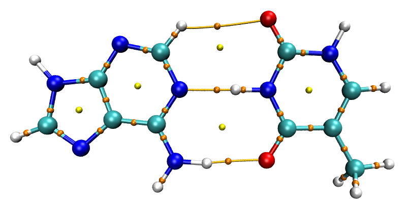
Then using the same way as Section 1.1 to perform IGMH calculation. Then in the console window of VMD, input source IGM_inter.vmd, then you will find \(\text{sign}(\lambda_2)\rho\) colored \(\delta g^\text{inter}\) isosurfaces have appeared, as shown below:

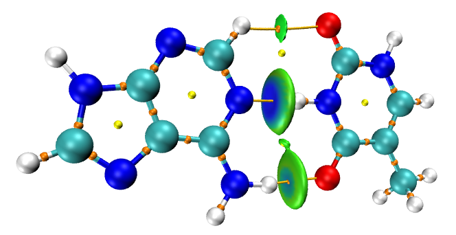
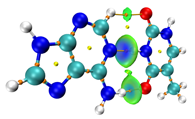
The \(\delta g^\text{inter}\) isosurface representing the N...H-N interaction is slightly thick, hence the orange sphere corresponding to the BCP is not visible in above map. You can try to slightly enlarge the size of the spheres, or make the isosurfaces transparent to solve this issue. To realize the later, you need do the following steps:

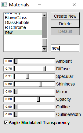
(1) Enter “Graphics” - “Materials”, select “Opaque”, and click “Create New” to create a copy.

(2) Rename the new material as “new”, then set the properties as follows:

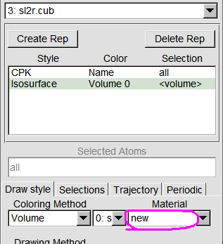
(3) Enter “Graphics” - “Representations”, set “Material” of the isosurface to “new”:

Now all BCPs can be directly observed:

1.6 Plot curve map and plane map of \(\delta g\)

Multiwfn is not only able to plot isosurface map of \(\delta g\) of various forms, but also to plot plane map and curve map. Here we plot \(\delta g\) in the plane of the AT dimer.

Boot up Multiwfn and input:

AT.wfn
4  // Main function 4: plot plane map
23  // The function to be plotted is IGMH δg
1  // Color-filled map
[Press ENTER button directly to use default grid setting]
0  // Set extension distance (see Section 3.5.2 of Multiwfn manual for detail)
1.5  // Extension distance is set to be 2.5 Bohr, which is suitable for present case
1  // XY plane
0  // Z=0

Click right mouse button on the window that pops up to close it, then input:

4  // Enable showing atom labels
1  // Red
8  // Enable showing bonds
14  // Brown
1  // Set lower and upper limits of color scale
0,0.1
-1  // Replot the map

Now you can see the following map:

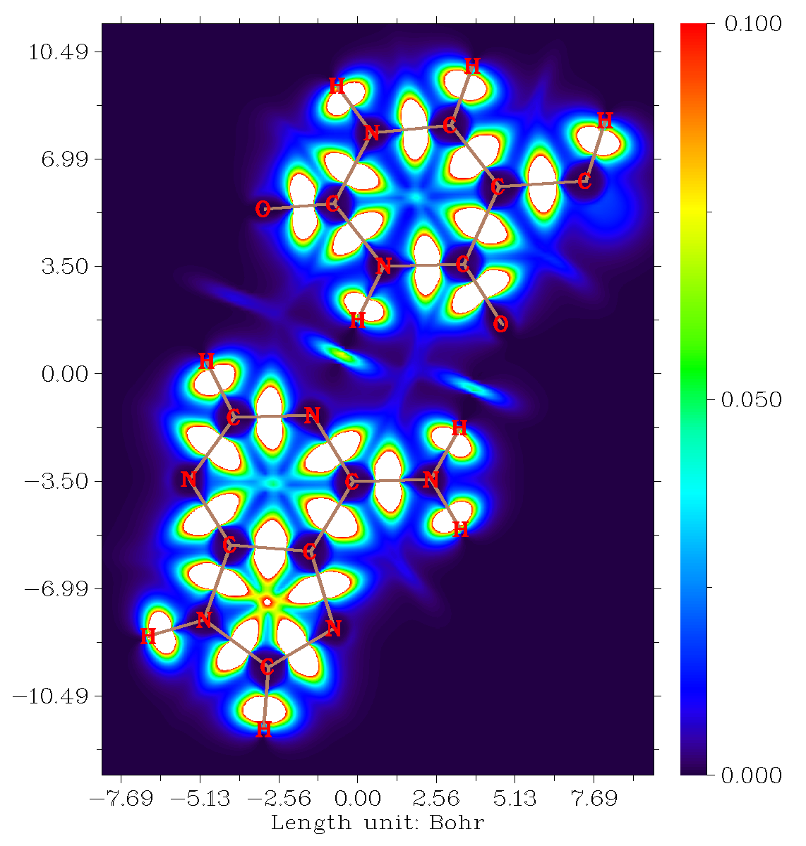
It can be seen that in the chemical bond regions, the \(\delta g\) is very large (the color is white because the value exceeds upper limit of color scale). You can also find that the \(\delta g\) in the region of N-H...N is larger than that of N-H...O. The \(\delta g\) in the C-H...O interaction area is trivial.

You can use many options in the post-process menu of the main function 4 to further improve graphical effect of the map. Also note that Multiwfn can plot many other kinds of plane map, such as contour line map and relief map. See abundant examples in Section 4.4 of Multiwfn manual for details.

Next, we plot curve map of \(\delta g\) along the line between H25 and N30, which are involved in the N19-H25...N30 interaction. Return to main menu of Multiwfn, then input:

3  // Output and plot specific property in a line
23  // The function to be plotted is IGMH δg
1  // Input index of two atoms to define a line
25,30  // Plot between atom 25 and atom 30

Now you can see the following map:

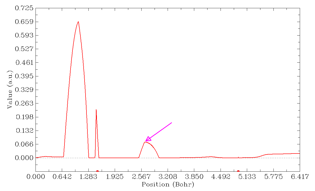
The two red points at the bottom of the map are nuclear positions of atoms H25 and N30, respectively. The position indicated by the pink arrow (manually labelled by me) is the maximum of \(\delta g\) corresponding to the H-bond interaction. To obtain its exact value, we close the map, then choose option “6 Find the positions of local minimum and maximum” in post-process menu, you will see position and value of all maxima and minima in the line:

[ignored...]
Maximum X (Bohr):    2.117506  Value:    0.12623326E-03
Minimum X (Bohr):    2.181673  Value:    0.12403025E-03
Maximum X (Bohr):    2.650091  Value:    0.76911821E-01
Minimum X (Bohr):    3.146314  Value:    0.86874146E-03
[ignored...]

It can be seen that the exact value corresponding to the peak of our interest is 0.0769 a.u., which is very close to the \(\delta g(\text{BCP})\) of the N...H-N interaction we obtained earlier (0.0772 a.u.).

There are also other peaks in the above curve map, they will not be mentioned here since they are not what we are really interested in.

1.7 Plot plane map of \(\delta g^\text{inter}\)

Next, I illustrate how to use Multiwfn to plot plane map of \(\delta g^\text{inter}\) in the plane of AT base pair. \(\delta g^\text{inter}\) in Multiwfn corresponds to the 91th user-defined function (as mentioned in Section 2.7 of Multiwfn manual). So, in order to plot it, we need to open settings.ini file of Multiwfn, change the “iuserfunc” parameter to 91, then save the file. After that, boot up Multiwfn and input:

AT.wfn
1000  // A hidden function
16  // Define one or two fragments for special purpose
2  // Define two fragments
15-29  // Atomic indices of fragment 1
1-14,30  // Atomic indices of fragment 2
4  // Plot plane map
100  // The function to be plotted is user-defined function, which corresponds to IGMH δg_inter currently
1  // Color-filled map
[Press ENTER button directly to use default grid setting]
0  // Set extension distance
1.5  // Extension distance is set to be 2.5 Bohr, which is suitable for present case
1  // XY plane
0  // Z=0

Then close the graph just shown on screen, and use various options in the post-process menu to improve graphical effect. In particular, the upper limit of color scale should be changed to 0.1, so that \(\delta g^\text{inter}\) in intermolecular interaction region can be exhibited clearly. Then you will see:

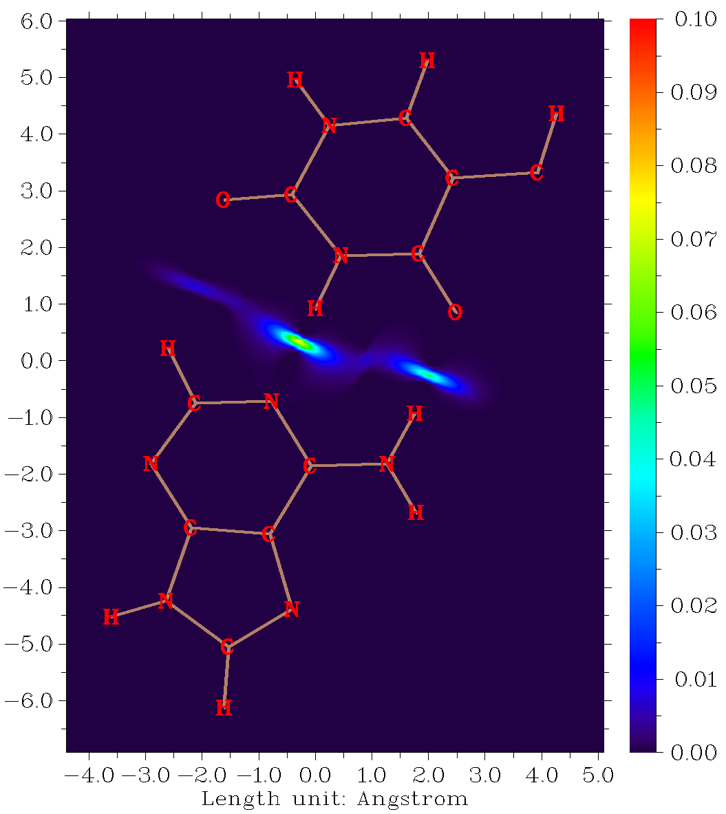
You can also plot curve map of \(\delta g^\text{inter}\) using similar way as last section, the only difference is that when Multiwfn asks you to select the function to be plotted, you should select “100 User-defined function”.