2. Example of more than two fragments: Oxazolidinone trimer

In this example, I will illustrate the flexibility of IGMH module in partitioning fragments. Oxazolidinone trimer will be taken as example, the geometry was taken from J. Chem. Theory Comput., 11, 3065 (2015) and is shown below. The wavefunction file is oxazolidinone_trimer.wfn in this tutorial package, which was generated at \(\omega\)B97XD/6-311G* level by single point calculation.

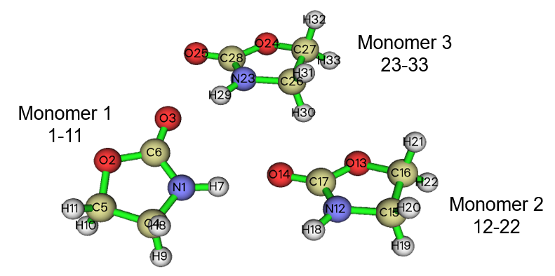
We first use IGMH to study interaction between monomer 2 and monomer 3. Boot up Multiwfn and input:

oxazolidinone_trimer.wfn
20  // Visual study of weak interaction
11  // IGMH analysis
2  // Define two fragments
12-22  // Define monomer 2 as fragment 1
23-33  // Define monomer 3 as fragment 2
11  // Select a batch of atoms, set extension distance and grid spacing (we use this mode to define grid because we are studying a subset of the whole system. This mode can avoid grid points appearing in irrelevant areas to a large extent and thus saving calculation time)
12-33  // Union of monomer 2 and monomer 3. Grid points will only occur around this part
1  // Extension distance. 1 Bohr is fully adequate in the present case, since the interaction between the two monomers only occur in their middle region
0.15  // Grid spacing (Bohr)
3  // Output cube files to current folder

Then move the newly generated dg_inter.cub and sl2r.cub to VMD folder, and also copy the IGM_inter.vmd script to VMD folder as mentioned in the last section. Then boot up VMD and input source IGM_inter.vmd in VMD console window, and then change the isovalue of \(\delta g^\text{inter}\) to 0.005, you will see:

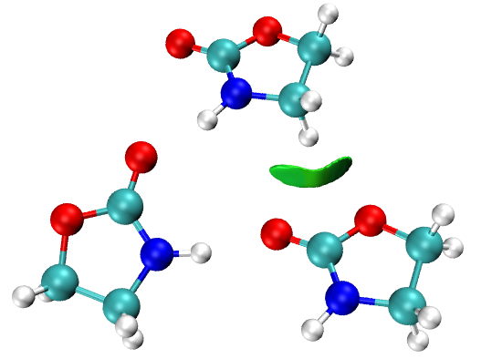
Clearly, only interaction between the specific two fragments is revealed.

Similarly, you can then plot the IGMH map between monomer 1 and monomer 3, by inputting the following commands:

0  // Return to interface of main function 20
11  // Enter IGMH analysis module again
2  // Two fragments
1-11  // Define monomer 1 as fragment 1
23-33  // Define monomer 3 as fragment 2
11  // Select a batch of atoms, set extension distance and grid spacing
1-11,23-33
1  // Extension distance of 1 Bohr
0.15  // Grid spacing of 0.15 Bohr

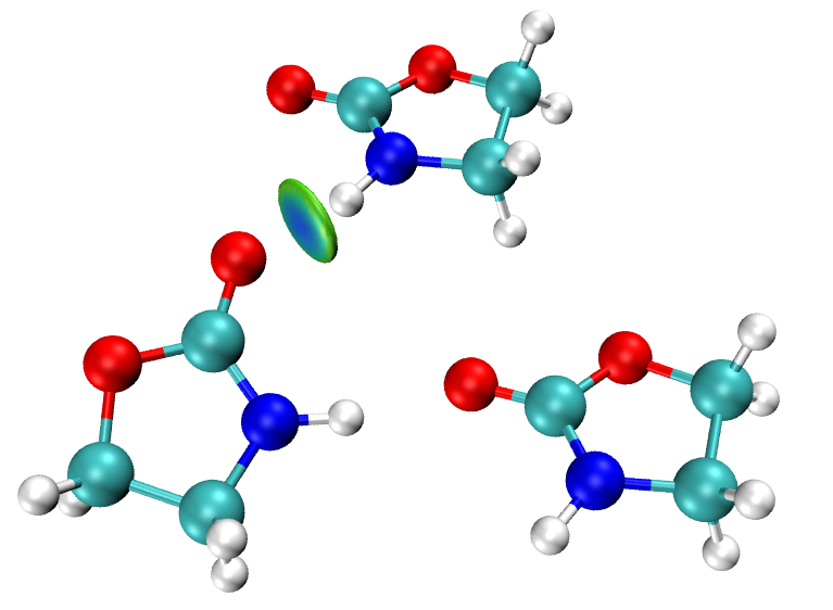
Then export .cub files and use VMD to plot via IGM_inter.vmd, you will see the following map, which only reveals the H-bond interaction between the two selected monomers:

By the way, if you want to visualize the spatial range of calculated grid data, you can visualize \(\delta g^\text{inter}\) via option “4 Show isosurface of grid data” in the post-process menu as illustrated in last section, then at the right side of the GUI window select “Show data range” check box, then you will see:

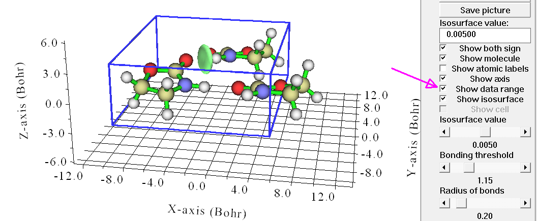
The blue box portrays the boundary of the grid data. As you can see, the spatial range of our calculated grid data is basically suitable. If the range is too narrow, the interested isosurfaces may be truncated, while if the range is too wide, a lot of calculation time will be wasted because many grid points appear in meaningless areas.

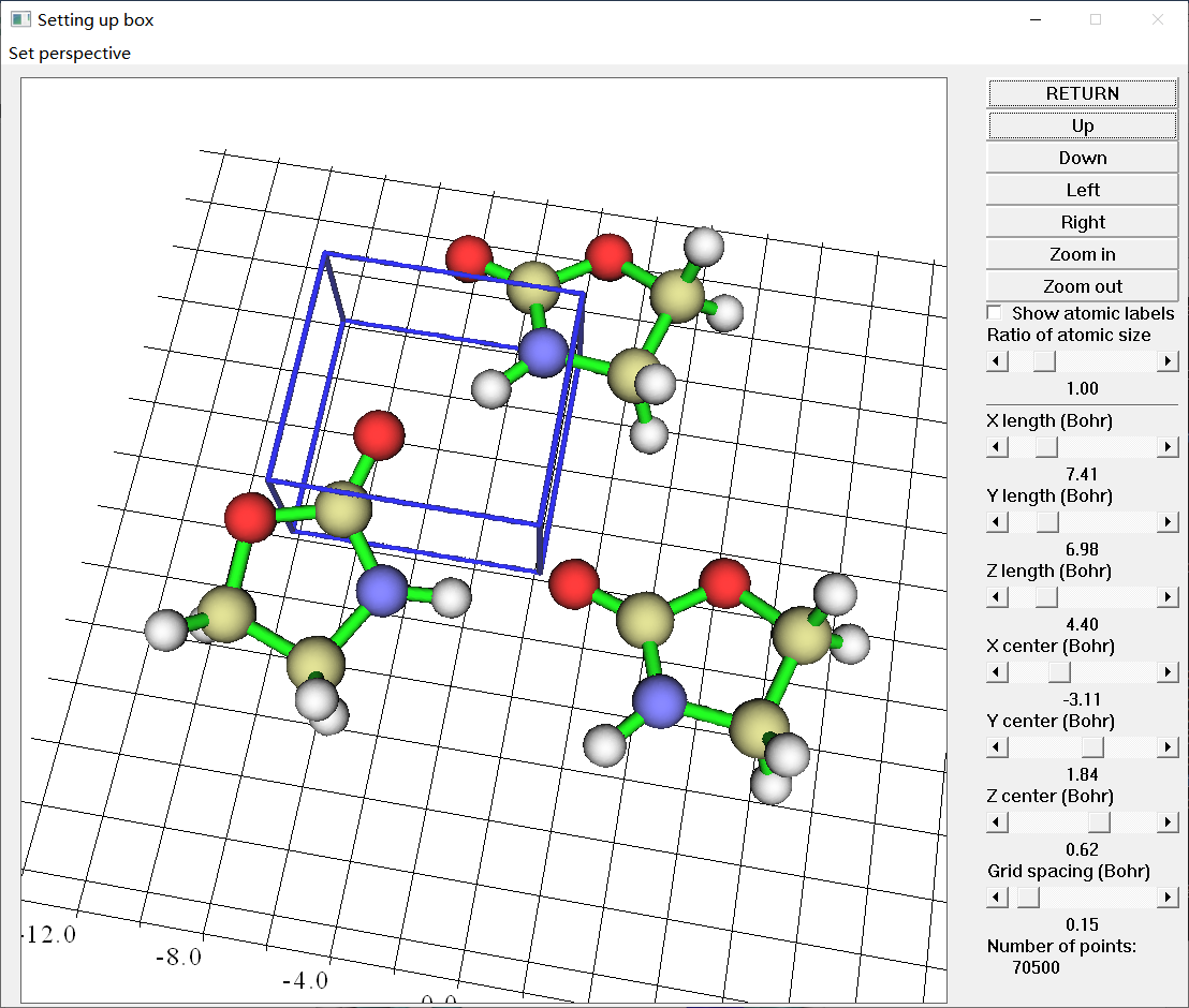
If you want to visually and accurately control the grid data range, it is advised to use mode “10 Set box of grid data visually using a GUI window” in grid setting interface. A screenshot of this mode is shown below. You can use corresponding widgets to carefully adjust box size and translate the box so that the range of the grid data to be calculated only encloses the region containing possibly interested interactions. For example, the box shown in the screenshot below encloses the region where the \(\delta g^\text{inter}\) isosurface corresponding to the H-bond may occur, therefore the number of points to be calculated is maximally reduced.

Finally, we study total interactions between the three monomers. Boot up Multiwfn and input:

oxazolidinone_trimer.wfn
20  // Visual study of weak interaction
11  // IGMH analysis
3  // Define three fragments
1-11  // Define monomer 1 as fragment 1
12-22  // Define monomer 2 as fragment 2
23-33  // Define monomer 3 as fragment 3
4  // Input the number of points or grid spacing in X,Y,Z, covering whole system
0.15  // Grid spacing of 0.15 Bohr

Then export .cub files and use the IGM_inter.vmd script to plot \(\delta g^\text{inter}\) isosurfaces in VMD. After manually changing the isovalue to 0.005 a.u., you will see:

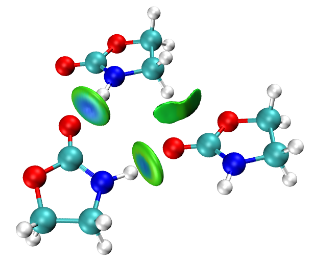
Clearly, all interactions among the three molecules have been nicely revealed.

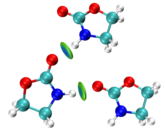
By the way, if you totally define two fragments, the first one corresponds to monomer 1 (atoms 1-11), and the second one corresponds to monomer 2 + monomer 3 (atoms 12-33), finally you will obtain the following map, which only reveals the two H-bonds between monomer 1 and the other two monomers:

In summary, this example fully illustrates how flexible the IGMH analysis in Multiwfn is!