3. Examples
In this section several examples are given, by following the examples one by one you can quickly understand how to utilize various features of Shermo to solve practical problems.
3.1 Calculating common thermodynamic quantities
In this section, I will take output file of frequency analysis for H₂CO by Gaussian 16 as example to describe how to use Shermo very easily to compute common thermodynamic quantities. This file is example\G16_H2CO_freq.out.
We will calculate data at 350 K, and we will employ frequency scale factors to eliminate systematical error. As can be seen from the Gaussian output file, the frequency analysis was conducted at B3LYP/6-31G* level (the geometry has been optimized at the same level before). According to Table 10 of J. Phys. Chem., 100, 16502 (1996), at this level the scale factor for ZPE is 0.9806, and the factors for entropy and heating contribution to internal energy are 1.0015 and 0.9989, respectively. Since the latter two are very close to 1, we simply approximate them as 1.0.
Open the settings.ini file in Shermo folder by text editor, change the value after "T=" to 350, change the value after "sclZPE=" to 0.9806, and change the value after “ilowfreq=” to 0 (using RRHO model in this example, which is the same as most quantum chemistry codes like Gaussian, but not as good as quasi-RRHO when there are low-frequencies, see next section). Note that there must be a space between the value and the equal sign. Finally, save the file.
I assume that you are using Windows system, double-clicking the "Shermo.exe" icon to boot up it, then you will see the parameters for current calculation:
Running parameters:
Printing individual contribution of vibration modes: No
Temperature:     350.000 K
Pressure:          1.000 atm
Scale factor of vibrational frequencies for ZPE:        0.9806
Scale factor of vibrational frequencies for U(T)-U(0):  1.0000
Scale factor of vibrational frequencies for S(T):       1.0000
Scale factor of vibrational frequencies for CV:         1.0000
Low frequencies treatment: Harmonic approximation
Then input the path of input file, namely example\G16_H2CO_freq.out. You can also directly drag icon of this file to the window of Shermo, the path will be automatically generated. After pressing ENTER button, Shermo will start to carry out calculation.
Shermo first prints molecular information, as shown below. I suggest you always check this part to guarantee that the running is meaningful. As you can see, the molecular information is fully correct. The electronic energy, spin multiplicity, atom masses and vibrational frequencies are directly loaded from Gaussian output file, the point group is determined by Shermo according to the geometry; the moments of inertia, rotational constants and temperatures are calculated based on geometry and atomic masses.
                      ======= Molecular information =======
Electronic energy:     -114.54925400 a.u.
Spin multiplicity:  1
Atom    1 (C )   Mass:   12.000000 amu
Atom    2 (H )   Mass:    1.007830 amu
Atom    3 (O )   Mass:   15.994910 amu
Atom    4 (H )   Mass:    1.007830 amu
Total mass:       30.010570 amu

Point group: C2v
Rotational symmetry number:  2
Principal moments of inertia (amu*Bohr^2):
     6.337337     46.220300     52.557637
Rotational constants relative to principal axes (GHz):
   284.779127     39.046506     34.338325
Rotational temperatures (K):   13.667227    1.873935    1.647978
This is not a linear molecule

There are     6 frequencies (cm^-1):
 1210.2  1273.5  1544.3  1819.4  2887.7  2945.7
Next, you can find contribution to various thermodynamic data by translation. The result is given in two common units. The "NA" denotes Avogadro constant.
                         ======= Translation =======
Translational q:   5.810322E+30     q/NA:  9.648265E+06
Translational U:      4.365 kJ/mol      1.043 kcal/mol
Translational H:      7.275 kJ/mol      1.739 kcal/mol
Translational S:    154.502 J/mol/K    36.927 cal/mol/K  -TS:   12.92 kcal/mol
Translational CV:    12.472 J/mol/K     2.981 cal/mol/K
Translational CP:    20.786 J/mol/K     4.968 cal/mol/K
Then you can see rotation contribution. Since only for translation, the U differs to H and CV differs to CP, therefore contributions to H and CP from rotation are not explicitly shown.
                         ========= Rotation ========
Rotational q:     8.932107E+02
Rotational U:      4.365 kJ/mol      1.043 kcal/mol    =H
Rotational S:     68.967 J/mol/K    16.484 cal/mol/K   -TS:   5.769 kcal/mol
Rotational CV:    12.472 J/mol/K     2.981 cal/mol/K   =CP
Next, you can find vibration contribution. As described in Section A.4, there are two forms of vibrational partition function, both of them are shown. The U(T)-U(0) term corresponds to heating contribution to internal energy (or enthalpy) from 0 to 350 K.
                         ======== Vibration ========
Vibrational q(V=0):     1.014709E+00
Vibrational q(bot):     3.798025E-11
Vibrational U(T)-U(0):     0.227 kJ/mol     0.054 kcal/mol   =H(T)-H(0)
Vibrational U:     68.738 kJ/mol     16.429 kcal/mol    =H
Vibrational S:      0.771 J/mol/K     0.184 cal/mol/K   -TS:   0.065 kcal/mol
Vibrational CV:     3.534 J/mol/K     0.845 cal/mol/K   =CP
Zero-point energy (ZPE):     68.51 kJ/mol,     16.37 kcal/mol    0.026094 a.u.
Electron excitation contribution is also outputted. However, for present system this part does not make sense, since only ground state is taken into account and this state is not degenerate.
                    ======== Electron excitation ========
Electronic q:     1.000000E+00
Electronic U:      0.000 kJ/mol      0.000 kcal/mol    =H
Electronic S:      0.000 J/mol/K     0.000 cal/mol/K   -TS:   0.000 kcal/mol
Electronic CV:     0.000 J/mol/K     0.000 cal/mol/K   =CP
At the end of the entire output you can find total result, see below. The partition function is product of all aforementioned contributions, all other quantities are sum of all aforementioned contributions.
                          ===========================
                          ========== Total ==========
                          ===========================
Total q(V=0):     5.266176E+33
Total q(bot):     1.971115E+23
Total q(V=0)/NA:   8.744690E+09
Total q(bot)/NA:   3.273112E-01
Total CV:      28.478 J/mol/K       6.806 cal/mol/K
Total CP:      36.792 J/mol/K       8.794 cal/mol/K
Total S:      224.240 J/mol/K      53.595 cal/mol/K    -TS:    18.758 kcal/mol
Zero point energy (ZPE):     68.511 kJ/mol     16.375 kcal/mol   0.026094 a.u.
Thermal correction to U:     77.469 kJ/mol     18.515 kcal/mol   0.029506 a.u.
Thermal correction to H:     80.379 kJ/mol     19.211 kcal/mol   0.030615 a.u.
Thermal correction to G:      1.895 kJ/mol      0.453 kcal/mol   0.000722 a.u.
Electronic energy:       -114.5492540 a.u.
Sum of electronic energy and ZPE, namely U/H/G at 0 K:      -114.5231595 a.u.
Sum of electronic energy and thermal correction to U:       -114.5197478 a.u.
Sum of electronic energy and thermal correction to H:       -114.5186394 a.u.
Sum of electronic energy and thermal correction to G:       -114.5485323 a.u.
As can be seen from above information, Shermo also outputs sum of electronic energy and various thermal corrections. For example, the "Sum of electronic energy and thermal correction to H" corresponds to the enthalpy of present molecule at current condition (350 K and 1 atm). However, this value is not accurate since electronic energy calculated at B3LYP/6-31G* level is poor. You can manually add the thermal corrections to a more accurate single point energy (e.g. CCSD(T)/cc-pVTZ) at current geometry to obtain better result.
Running under Linux
The way of running this example in Linux platform is mentioned below.
You can edit the settings.ini in aforementioned way, then enter the Shermo folder and run ./Shermo to boot up it, then input the path of input file. You can also specify the path of input file as argument, for example, ./Shermo example/G16_H2CO_freq.out.
If you hope Shermo can run in arbitrary directory, you should add below two lines into your ~/.bashrc file and re-enter the shell (the Shermo folder is assumed to be /sob/Shermo_2.0)
In this case, if settings.ini cannot be found in current folder, Shermo will try to locate it from /sob/Shermo_2.0 folder. If it still cannot be found, default parameters will be used.
Modification on settings.ini in fact can be avoided, since parameters can also be specified by arguments. To reproduce the present example, you can run below command
In this case temperature and scale factor for ZPE are explicitly specified, all other parameters will use the values defined in settings.ini; while if settings.ini cannot be found, default parameters will be used.
If you want, you can use > operator to redirect all outputted information from screen to a plain text file.
3.2 Printing contribution of individual vibrational modes
In this example, we check contribution of individual vibrational modes to thermodynamic quantities, this is useful to understand the role played by various modes. The input file is example\ORCA_ethanol_optfreq.out, which is output file of optimization with frequency analysis of ORCA 4.2 program for ethanol, the B3LYP/6-31G* level was employed. In the settings.ini, we set "sclZPE" to 0.9806 as the last example, set "T" to 298.15, and set "prtvib" to -1.
Now, use Shermo to analyze the ORCA output file, then not only thermodynamic data are printed on screen, but also a file named vibcontri.txt is generated in current folder, its content is shown below:
Note: The wavenumbers shown below are unscaled ones

  Mode  Wavenumber    Freq        Vib. Temp.    q(V=0)        q(bot)
          cm^-1        GHz            K
    1     247.04   0.74061E+04      355.44    1.43589955    0.79114346
    2     297.95   0.89323E+04      428.68    1.31138455    0.63901869
    3     417.19   0.12507E+05      600.24    1.15414458    0.42178802
...ignored
   19    3127.85   0.93771E+05     4500.27    1.00000028    0.00052769
   20    3130.25   0.93843E+05     4503.73    1.00000028    0.00052465
   21    3746.34   0.11231E+06     5390.14    1.00000001    0.00011865

  Mode  Wavenumber     ZPE      U(T)-U(0)    U(T)      CV(T)       S(T)
          cm^-1      kcal/mol   kcal/mol   kcal/mol  cal/mol/K  cal/mol/K
    1     247.04     0.34631    0.30789    0.65420    1.76768    1.75161
    2     297.95     0.41768    0.26526    0.68294    1.67754    1.42839
    3     417.19     0.58483    0.18386    0.76870    1.43290    0.90157
...ignored
   19    3127.85     4.38474    0.00000    4.38474    0.00013    0.00001
   20    3130.25     4.38810    0.00000    4.38811    0.00012    0.00001
   21    3746.34     5.25176    0.00000    5.25176    0.00001    0.00000
In the output, contribution to various thermodynamic quantities due to vibration has been clearly decomposed as contributions from various modes. Note that the values under "Wavenumber" and "Freq" labels are the original frequencies (i.e. without applying scale factor). From the data it can be seen that the lower the frequency of a mode, the higher its contribution to U(T)-U(0), CV and S. In contrast, the higher the frequency of a mode, the larger its contribution to ZPE and U(T).
If you prefer to use Shermo in command-line environment, you can also use -prtvib -1 argument to request Shermo output the vibcontri.txt.
3.3 Using quasi-RRHO treatment for low-frequencies
As described in Section A.4, if your system contains many low-frequency modes, it is highly suggested to deal with them using quasi-RRHO model instead of RRHO (i.e. harmonic approximation) to obtain more reasonable entropy, U(T)-U(0) and CV. In this example, we will calculate thermodynamic data for remdesivir, which is a specific medicine against COVID-19 virus. Its most stable conformation determined by the powerful conformation and configuration search program Molclus (http://www.keinsci.com/research/molclus.html) is shown below. The output file of optimization with frequency analysis task at B3LYP-D3(BJ)/6-31G* level of Gaussian 16 is example\G16_remdesivir_optfreq.out.
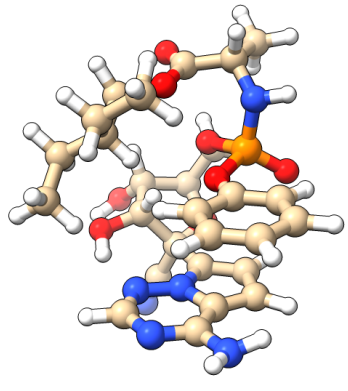
We first conduct analysis at standard condition with RRHO treatment like previous examples (using “ilowfreq= 0”). Notice that from output you can find that there are many low frequencies, as shown below. The contribution to S, U(T)-U(0) and CV from the modes lower than 150 cm⁻¹ is usually unable to be well represented by RRHO model.
There are   225 frequencies (cm^-1):
    8.7    20.0    32.1    33.3    38.1    41.0    45.9    53.2    65.1
   70.3    74.4    75.6    79.9    87.4    92.8   104.4   108.3   117.6
  123.9   131.4   139.1   150.3   155.5   165.6   175.7   184.9   190.8
...ignored
The output of vibration part is
                         ======== Vibration ========
Vibrational q(V=0):     2.077261E+18
Vibrational q(bot):     7.935674-270
Vibrational U(T)-U(0):   100.764 kJ/mol    24.083 kcal/mol   =H(T)-H(0)
Vibrational U:   1709.523 kJ/mol    408.586 kcal/mol    =H
Vibrational S:    688.648 J/mol/K   164.591 cal/mol/K   -TS:  49.073 kcal/mol
Vibrational CV:   632.893 J/mol/K   151.265 cal/mol/K   =CP
Zero-point energy (ZPE):   1608.76 kJ/mol,    384.50 kcal/mol    0.612744 a.u.
Then, we change the "ilowfreq" in settings.ini to 1, namely raising frequencies lower than a specific threshold to this value. The threshold is controlled by "ravib" parameter, which is 100 by default. The output in this case is
                          ======== Vibration ========
 Note:   15 low frequencies are raised to 100.0 cm^-1 during calculating S, U(T)
-U(0), CV and q
 Vibrational q(V=0):     1.163912E+14
 Vibrational q(bot):     8.570305-275
 Vibrational U(T)-U(0):    97.144 kJ/mol    23.218 kcal/mol   =H(T)-H(0)
 Vibrational U:   1705.902 kJ/mol    407.720 kcal/mol    =H
 Vibrational S:    595.110 J/mol/K   142.235 cal/mol/K   -TS:  42.407 kcal/mol
 Vibrational CV:   631.362 J/mol/K   150.899 cal/mol/K   =CP
 Zero-point energy (ZPE):   1608.76 kJ/mol,    384.50 kcal/mol    0.612744 a.u.
Next, we use Grimme's quasi-RRHO treatment of entropy for this system. Change the "ilowfreq" to 2 and redo the calculation, the result is
                         ======== Vibration ========
Vibrational q(V=0):     2.077261E+18
Vibrational q(bot):     7.935674-270
Vibrational U(T)-U(0):   100.764 kJ/mol    24.083 kcal/mol   =H(T)-H(0)
Vibrational U:   1709.523 kJ/mol    408.586 kcal/mol    =H
Vibrational S:    608.552 J/mol/K   145.447 cal/mol/K   -TS:  43.365 kcal/mol
Vibrational CV:   632.893 J/mol/K   151.265 cal/mol/K   =CP
Zero-point energy (ZPE):   1608.76 kJ/mol,    384.50 kcal/mol    0.612744 a.u.
Some data are summarized in the following table. Note that the Grimme's quasi-RRHO is only applied to entropy and thus U(T)-U(0) and CV are not affected.
| Model | U(T)-U(0) (kcal/mol) | -TS (kcal/mol) | CV (cal/mol/K) |
|---|---|---|---|
| RRHO | 24.1 | 49.1 | 151.3 |
| Raising low freq. | 23.2 | 42.4 | 150.9 |
| Grimme | 24.1 | 43.4 | 151.3 |
From the table it can be seen that the U(T)-U(0) and CV calculated under RRHO and quasi-RRHO (with ilowfreq=1) do not differ with each other significantly, however, both the two quasi-RRHO models altered the -TS term of RRHO by more than 10%, rendering importance of applying quasi-RRHO model for large and flexible systems like this. Since the two quasi-RRHO models result in similar result, both of them may be used in practice. In my opinion, using Grimme's model (ilowfreq=2) is more ideal, since it has relatively more rigorous physical basis.
In command-line environment, you can also activate the quasi-RRHO treatment in calculation by adding -lowfreq 1 or -ilowfreq 2 argument.
3.4 Scanning temperature and pressure
In this example, we study variation of various thermodynamic quantities with respect to temperature and pressure. The input file is examples\NWChem_NH2COH_optfreq.out, which is optimization with frequency analysis task at B3LYP/6-31G* level by NWChem for NH₂COH. Again, we employ scale factor of 0.9806 for ZPE by modifying "sclZPE" parameter in settings.ini. All other parameters keep default value.
Initially, we scan temperature from 50 to 1000 K with stepsize of 10 K, therefore we modify the line defining temperature in settings.ini as "T= 50,1000,10". Start Shermo calculation as usual, then you will find scan_SCq.txt has been generated in current folder, which contains \(S\), \(C_{\rm V}\), \(C_{\rm P}\), \(q^{(\rm V=0)}/N_{\rm A}\) and \(q^{(\rm bot)}/N_{\rm A}\). Its content is
Unit of S, CV and CP is cal/mol/K, q(V=0)/NA and q(bot)/NA are dimensionless

     T(K)     P(atm)      S         CV        CP       q(V=0)/NA      q(bot)/NA
    50.000     1.000    45.106     7.286     9.273   1.012978E+008   7.711220E-117
    60.000     1.000    46.813     7.456     9.443   2.219362E+008   8.206613E-096
    70.000     1.000    48.278     7.574     9.561   4.353700E+008   9.611775E-081
    80.000     1.000    49.561     7.661     9.648   7.865970E+008   2.097511E-069
    90.000     1.000    50.701     7.735     9.722   1.333255E+009   1.479802E-060
...ignored
Another file generated in current folder is scan_UHG.txt, which contains thermal corrections to U, H and G, as well as sum of each of them and electronic energy:
Unit of Ucorr, Hcorr and Gcorr is kcal/mol, unit of U, H and G is a.u.

     T(K)     P(atm)    Ucorr     Hcorr     Gcorr            U                H                G
    50.000     1.000    28.170    28.269    26.014      -169.843950      -169.843791      -169.847386
    60.000     1.000    28.244    28.363    25.554      -169.843832      -169.843642      -169.848118
    70.000     1.000    28.319    28.458    25.079      -169.843712      -169.843491      -169.848876
    80.000     1.000    28.395    28.554    24.589      -169.843591      -169.843338      -169.849656
...ignored
Based on the two files, you can easily plot variation curve of various quantities with respect to temperature. For example, the below map was plotted by Origin:
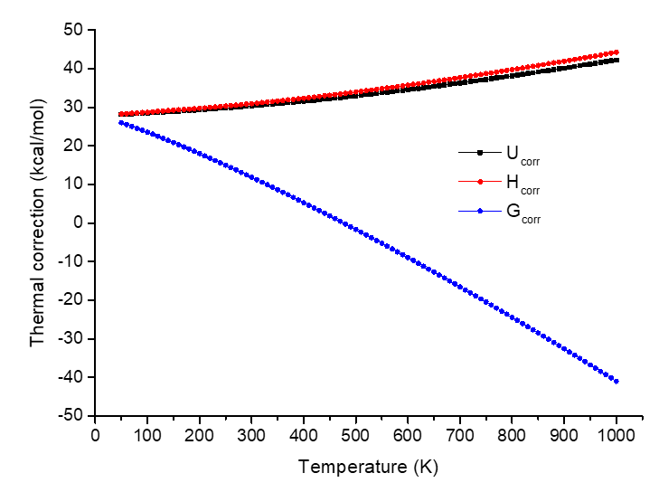
The Gcorr decreases with increase of temperature due to the -TS term and the fact that S is a positive value.
Similarly, you can set the "P" parameter in settings.ini to e.g. "P= 0.5,20,0.1" to scan pressure from 0.5 to 20 atm with stepsize of 0.1 atm.
If you specify lower and upper limits as well as stepsize for both "T" and "P", then Shermo will do two-dimension scan. For example, if you set
then the resulting scan_SCq.txt will be
     T(K)     P(atm)      S         CV        CP       q(V=0)/N       q(bot)/N
   250.000     0.600    62.407     9.953    11.940   2.790475E+11   4.187769E-14
   250.000     0.800    61.835     9.953    11.940   2.092856E+11   3.140827E-14
   250.000     1.000    61.392     9.953    11.940   1.674285E+11   2.512662E-14
   260.000     0.600    62.879    10.149    12.136   3.404227E+11   4.603420E-13
   260.000     0.800    62.307    10.149    12.136   2.553170E+11   3.452565E-13
   260.000     1.000    61.864    10.149    12.136   2.042536E+11   2.762052E-13
   270.000     0.600    63.341    10.349    12.336   4.128023E+11   4.274044E-12
   270.000     0.800    62.769    10.349    12.336   3.096017E+11   3.205533E-12
   270.000     1.000    62.326    10.349    12.336   2.476814E+11   2.564426E-12
...ignored
3.5 Using electronic energy at better level
In the previous examples, the electronic energy loaded from input file was employed. However, in practical calculations of thermodynamic data, commonly electronic energy evaluated at a better level via an additional single point task should be used, since U, H and G are dominated by electronic energy, while accuracy of electronic energy is significantly more sensitive to quality of calculation level than optimization and frequency analysis tasks. In this section, the ethyl radical will be taken as example to illustrate how to use electronic energy evaluated at a better level in thermochemistry calculation.
This time we perform optimization and frequency analysis at a more robust level than earlier examples, namely B2PLYP-D3(BJ)/cc-pVTZ. The output file is example\C2H5_optfreq.out. The optimal ZPE scale factor for this level is reported to be 0.9830 in J. Chem. Theory Comput., 12, 3774 (2016), while the scale factor for S and U(T)-U(0) can be still approximated to be 1.0. Based on the optimized geometry a single point task was conducted, the electronic energy calculated at the very accurate CCSD(T)/cc-pVQZ level was found to be -79.0257037 a.u.
In the settings.ini, we change the "sclZPE" parameter to 0.983, change the "ilowfreq" to 2 to use Grimme's quasi-RRHO treatment since this system has a low-frequency mode (rotation of methyl group), and set "E" to -79.0257037.
Now boot up Shermo and use the C2H5_optfreq.out as input file, the result is
Electronic energy:        -79.0257037 a.u.
Sum of electronic energy and ZPE, namely U/H/G at 0 K:        -78.9670179 a.u.
Sum of electronic energy and thermal correction to U:         -78.9630711 a.u.
Sum of electronic energy and thermal correction to H:         -78.9621269 a.u.
Sum of electronic energy and thermal correction to G:         -78.9910754 a.u.
Since the current electronic energy is highly accurate, the ZPE scale factor has been taken into account, and quasi-RRHO treatment is employed, the resulting U, H and G shown above should be fairly reliable.
If you prefer to use command-line mode to run Shermo, you can input
Customizing electronic energy via shm file
In Shermo there is another way of employing electronic energy calculated at other level than frequency analysis, namely utilizing .shm file as input file, as illustrated below.
We set the "outshm" in settings.ini to 1, in this case Shermo will generate a .shm file when output file of quantum chemistry program is used as input file. The shm file contains everything that needed by Shermo to compute thermodynamic data and thus can then be used as input file. You can manually make various modifications on .shm file.
Now, boot up Shermo and use the example\C2H5_optfreq.out as input file, then example\C2H5_optfreq.shm will be generated. Open this file by text editor, change the value under the *E label as -79.0257037. Now the file content should be
*E  //Electronic energy (a.u.)
-79.0257037
*wavenum  //Wavenumbers (cm-1). Negative value means imaginary frequency
  120.0311
  479.5592
  818.5287
  990.8014
 1073.5208
 1207.5756
 1413.2669
 1483.9190
 1497.2870
 1498.1094
 2985.2923
 3070.3466
 3114.8558
 3174.7147
 3277.7883
*atoms  //Information of all atoms: Name, mass (amu), X, Y, Z (Angstrom)
C    12.000000    0.055460   -0.706009    0.000000
H     1.007830   -0.452385   -1.093686    0.882849
H     1.007830    1.060514   -1.146711    0.000000
H     1.007830   -0.452385   -1.093686   -0.882849
C    12.000000    0.103111    0.777922    0.000000
H     1.007830    0.193594    1.327564   -0.923232
H     1.007830    0.193594    1.327564    0.923232
*elevel  //Energy (eV) and degeneracy of electronic energy levels
    0.000000   2
Note that the data under *elevel label represents electronic energy levels. Since only ground state is considered, the excitation energy is 0.000000 eV. The current system is doubly degenerate due to spin multiplicity of 2, therefore there is a "2" in this line. If you use this .shm file as input file of Shermo, you will obtain exactly the same result as before.
3.6 Consideration of degeneracy of ground state and spin-orbit coupling splitting
When ground state has spatial degeneracy, its influence on entropy and free energy must be properly taken into account. In this section I make a few remarks about this point.
The *elevel field in .shm file records all electronic levels that considered in the calculation. Usually you do not need to manually modify this field, because:
(1) Separations between ground state and excited states are commonly as large as a few electronvolts, thus electron excitations do not detectably contribute to thermodynamic data.
(2) Commonly degeneracy of ground state is only due to electron spin multiplicity, which is directly loaded by Shermo from input file, thus this point is automatically taken into account.
However, for some single atom systems and diatom systems, degeneracy also comes from spatial part of wavefunction. In addition, spin-orbit coupling (SOC) effect can split the degenerate ground states and result in very low-lying excited states. Below I give two instances to illustrate how to consider this point.
OH radical
The ground state of OH radical (\(^2\Pi\) state) has spin multiplicity of 2 and spatial degeneracy of 2, therefore the total degeneracy of this state is \(2\times 2=4\). So, the content under the *elevel label should be
The result of electron excitation part of output is
Electronic q:    4.000000E+000
Electronic U:      0.000 kJ/mol      0.000 kcal/mol    =H
Electronic S:     11.526 J/mol/K     2.755 cal/mol/K   -TS:   0.821 kcal/mol
Electronic CV:     0.000 J/mol/K     0.000 cal/mol/K   =CP
While if you hope to take SOC effect into account to obtain more rigorous result, the four degenerate states will split into two doubly degenerate states with energy separation of 139.2 cm⁻¹ (0.0172 eV), in this case the content of the *elevel field should be changed to
Now the result is
Electronic q:    3.023977E+000
Electronic U:    561.954 kJ/mol    134.310 kcal/mol    =H
Electronic S:     11.085 J/mol/K     2.649 cal/mol/K   -TS:   0.790 kcal/mol
Electronic CV:     0.835 J/mol/K     0.199 cal/mol/K   =CP
The comparison shows that SOC effect only marginally affects thermodynamic data, the -TS only changed by 0.03 kcal/mol.
Fluorine atom
Ground state of fluorine atom is (\(^2P\)), its spin multiplicity is 2 while spatial degeneracy is 3 because fluorine atom has three 2p orbitals, the unpaired electron may occupy any of them. To represent this fact, the content of the *elevel field should be
Due to SOC effect, the six degenerate states are split to a J=3/2 state of degeneracy of four (ground state) and a J=1/2 state of degeneracy of two, whose excitation energy is 404.141 cm⁻¹ (0.050107 eV). To account for this situation, the content of *elevel should be
Comparison of different considerations of ground state degeneracy is given below, where T=298.15 K and n stands for degeneracy
| Spin degeneracy (n=2) | Spin + spatial degeneracy (n=6) | with SOC (n=4+2) | |
|---|---|---|---|
| q | 2 | 6 | 4.3 |
| S (J/mol/K) | 5.76 | 14.90 | 13.17 |
| -TS (kJ/mol) | 0.41 | 1.06 | 0.94 |
As can be seen, including spatial degeneracy has crucial influence on Gibbs free energy, which reflects by the -TS term. Clearly, spatial degeneracy should never be ignored if accuracy of the result is important. The SOC effect only slightly affects the -TS term (0.94 -1.06 = -0.12 kJ/mol), thus ignoring SOC effect is usually an acceptable approximation in the calculation of thermal correction to Gibbs free energy.
3.7 Calculate a batch of conformations and obtain conformation weighted thermodynamic data
The remdesivir molecule has been studied in Section 3.3. In fact, conformation search of the remdesivir by Molclus code yielded a batch of low energy conformations. In this example we will use Shermo to calculate thermodynamic data of all conformers at once and meantime obtain Boltzmann weighted result. For the three lowest conformers, the output files of optimization with frequency analysis task of Gaussian as well as output files of single point calculation of ORCA have been provided in "example\ensemble" folder. Since the frequency analyses were conducted at B3LYP-D3(BJ)/6-31G* level, we will use ZPE scale factor of 0.9806. The single point calculation was conducted at PWPB95-D3(BJ)/def2-QZVPP level with SMD solvation model, which is fairly robust. Again, since the remdesivir is quite flexible, we will use Grimme's quasi-RRHO treatment for entropy.
In the settings.ini file, we set "sclZPE" to 0.9806, set "ilowfreq" to 2, all other parameters keep default values. Then we create a file named list.txt with following content
example\ensemble\gau00001.out;-2321.367718855799
example\ensemble\gau00002.out;-2321.363532347723
example\ensemble\gau00003.out;-2321.369898466825
Each line contains path of an output file, the value after semicolon is the single point energy in a.u. evaluated at PWPB95-D3(BJ)/def2-QZVPP with SMD (if you do not explicitly specify the electronic energies, then the electronic energies loaded from the .out files will be used, which are poor).
Now run Shermo using the list.txt as input file, you will see below output information
 Processing example\ensemble\gau00001.out... (    1  of    3 )
 Processing example\ensemble\gau00002.out... (    2  of    3 )
 Processing example\ensemble\gau00003.out... (    3  of    3 )

 #System       U               H               G             S          CV
              a.u.            a.u.            a.u.        J/mol/K     J/mol/K
    1    -2320.713764    -2320.712819    -2320.821265     954.971     657.837
    2    -2320.709745    -2320.708801    -2320.817499     957.191     657.295
    3    -2320.715999    -2320.715054    -2320.822180     943.341     654.902

 System    1     Relative G=    2.401 kJ/mol     Boltzmann weight=  27.380 %
 System    2     Relative G=   12.289 kJ/mol     Boltzmann weight=   0.507 %
 System    3     Relative G=    0.000 kJ/mol     Boltzmann weight=  72.113 %

 Conformation weighted data:
 Electronic energy:     -2321.369269 a.u.
 U:     -2320.715355 a.u.
 H:     -2320.714411 a.u.
 G:     -2320.822488 a.u.
 S:       951.727 J/mol/K    Conformation entropy:     5.132 J/mol/K
 CV:      655.718 J/mol/K
 CP:      664.032 J/mol/K
It can be seen that various thermodynamic quantities for the three conformations are separately outputted, then the Gibbs free energies of the three systems relative the lowest one are shown, and meantime the Boltzmann weights estimated according to relative free energies are also given. Evidently conformer 3 plays a dominant role, while conformer 2 can be safely ignored (at least in the present condition, namely 298.15 K and 1 atm). Finally, conformation weighted thermodynamic data as well as conformation entropy are shown, see Section A.6 on how they are calculated. Note that the conformation entropy has already been considered in the value printed after "S:".
Note that there is an another way of realizing the present example. We create list.txt with below content:
Then change "outshm" in settings.ini to 1, then boot up Shermo and use the list.txt as input file, you will see
Processing example\ensemble\gau00001.out... (    1  of    3 )
Outputting data to example\ensemble\gau00001.shm
example\ensemble\gau00001.shm has been successfully generated
Processing example\ensemble\gau00002.out... (    2  of    3 )
Outputting data to example\ensemble\gau00002.shm
example\ensemble\gau00002.shm has been successfully generated
Processing example\ensemble\gau00003.out... (    3  of    3 )
Outputting data to example\ensemble\gau00003.shm
example\ensemble\gau00003.shm has been successfully generated
Now we have three .shm files corresponding to the three conformers. In order to use more accurate electronic energy, we copy the PWPB95-D3(BJ)/def2-QZVPP single point energies from the three ORCA output files to the corresponding .shm files. For example, the example\ensemble\orcaSP00001.out contains the energy of conformer 1, thus we copy the energy "-2321.367718855799" from it to the second line of example\ensemble\gau00001.shm. After modifying the three .shm files, we replace all ".out" in the list.txt with ".shm". Finally, use the list.txt as input file to run Shermo, you will obtain exactly the same result as before.
3.8 Consideration of variation of Gibbs free energy due to concentration change
Variation of Gibbs free energy caused by change of concentration at temperature T is
where \(c_A\) and \(c_B\) are concentrations of initial state and final state. respectively.
This change of G must be properly taken into account. In particular, when G of a molecule in solution is studied, it is usually given at concentration of 1 M, which is standard state concentration of solution phase. Via Shermo it is straightforward to convert the G at present concentration (namely c=P/RT according to ideal gas formula) to 1 M or other expected concentration.
As an example, the G obtained in the example of last section corresponds to concentration at gas phase standard state (since T and P are set to 298.15 K and 1 atm in settings.ini, respectively). To obtain the G corresponding to 1 M concentration (still at 298.15 K), we should change value of “conc” parameter in settings.ini from the default 0 to 1M. Then after running the example in last section again, at the end of output you will see
[ignored...]
G:     -2320.822488 a.u.
 S:       951.727 J/mol/K    Conformation entropy:     5.132 J/mol/K
 CV:      655.718 J/mol/K
 CP:      664.032 J/mol/K

 Present concentration (estimated by ideal gas model):  0.040874 mol/L
 Concentration specified by "conc" parameter:    1.000000 mol/L
 delta-G of conc. change:      7.926 kJ/mol      1.894 kcal/mol   0.003019 a.u.
 Weighted Gibbs free energy at specified concentration:      -2320.8194695 a.u.
It shows that the Gconc corresponding to changing from present state (0.040874 M) to the concentration specified by “conc” parameter (1 M) is 0.003019 a.u., adding it to the G in present state (2320.822488 a.u., the same as the last example) results in the G in 1M (G1M = 2320.8194695 a.u.). Usually, when G in solution is involved in study, such as calculating G of chemical reaction that occurs in solution, you should use G1M. Of course, you can also for example set “conc” to 2.4M if G corresponding to other concentration is needed.
PS: The 0.040874 M (mol/L) is calculated P/RT=101325/(8.314*298.15)/1000. Note that 1 atm=101325 Pa, R=8.314 J/mol/K, the 1000 is used to convert mol/m³ to mol/L.
Skill: Using shell script to invoke Shermo to deal with a batch of files
If you have a lot of files for which thermodynamic data are to be calculated, you can easily write a shell script to automatically invoke Shermo to calculate the data. For example, assume that you are using Linux platform (or under Windows platform but using WSL, cmder or Cygwin to simulate Bash shell), there are a batch of .out files, you want to calculate Gibbs free energy at standard condition for all of them, ZPE scale factor of 0.975 and Grimme's QRRHO treatment will be used, you can create a text file (for example getGall.sh) with the following content
#!/bin/bash
outname=Gall.txt
rm -f $outname
for inf in `ls -v *.out`
do
echo Processing ${inf} ...
echo ${inf} >> $outname
./Shermo ${inf} -sclZPE 0.975 -ilowfreq 2 | grep "Sum of electronic energy and thermal correction to G:" | cut -d: -f 2 >> $outname
done
echo "Data have been exported to $outname in current folder"
The content of this script is very easy to comprehend if you have basic knowledge about shell scripting. Put this shell script and Shermo executable file in the current folder, then run command ./getGall.sh, then all .out files will be processed by Shermo in turn, finally from the Gall.txt in current folder you can find the result, for example
Cs-atom-in.out
        -705.4867512 a.u.
Cs-ion-in.out
        -705.2690829 a.u.
Cs-ion-out.out
        -705.2490426 a.u.
K-atom-in.out
       -1285.2091502 a.u.
K-ion-in.out
       -1284.9920128 a.u.
K-ion-out.out
       -1284.9852452 a.u.
Please write your own scripts based on the above example to facilitate your practical researches. The scripts for extracting electronic energy, G, H and -TS terms for all .out files in current folder have already been provided as getEall.sh, getGall.sh, getHall.sh and get-TSall.sh in “examples” folder, respectively.