optDFTw: A program for tuning ω parameter of long-range corrected functionals
Introduction of ω tuning and optDFTw
Long-range corrected (LRC) density functionals, such as LC-ωPBE, LC-PBE, LC-PBE0, LC-BLYP, etc., have a key parameter, ω. These functionals could perform much better for a system if ω is specifically optimized (tuned) for this system, that means the optimal ω is highly system-dependent. A very popular approach for tuning ω is known as IP-tuning or gap-tuning, which makes satisfaction of Koopmans' theorem as good as possible by varying ω, the deviation to Koopmans' theorem is measured by J and J2 values:
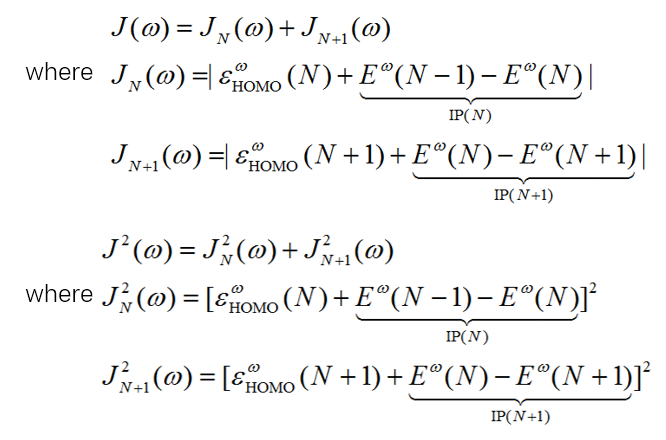
The physical rationale behind this method is that, for an exact exchange-correlation functional, the HOMO energy should be precisely equal to the ionization potential—exactly satisfying Koopmans' theorem. Once ω is tuned in this manner, LRC functionals can predict many properties quite well, such as excitation energies, (hyper)polarizabilities, fundamental gaps, and singlet-triplet energy splittings. See Acta Phys. -Chim. Sin., 32, 2197 (2016) DOI: 10.3866/PKU.WHXB201605301 for a review of ω tuning.
optDFTw is a code to make tuning the ω parameter as easy as possible for Gaussian users (currently G09 and G16 are formally supported) and ORCA users (at least compatible with 6.1.1; other versions were not tested). optDFTw iteratively optimizes ω by minimizing J2 (but J is also printed), convergence of ω can usually be reached in 10-20 iterations. In each iteration, Gaussian or ORCA is automatically invoked by optDFTw to calculate single point energy of N, N-1 and N+1 states, where N is the number of electrons at original state. Both neural and charged systems, as well as closed-shell and open-shell systems, are supported.
Another utility named scanDFTw is also provided along with optDFTw, it performs scan of ω in a specific range so that users can check how J and J2 varies with respect to ω.
Developer
Dr. Tian Lu (Contact: sobereva[at]sina.com. Beijing Kein Research Center for Natural Sciences, China)
Citation
If optDFTw is utilized in your work, please cite:
Download
Update History
2026-Oct-30Version 2.0: settings.ini file is introduced to more easily and flexibly control the calculation, which also makes charged systems and open-shell systems supported. ORCA is fully supported. Output information is improved, small bugs are fixed.
2016-Sep-20Version 1.0: Initial release.
Usage of optDFTw
1Gaussian or ORCA should have been properly installed on your machine.
2Decompressing optDFTw package and enter its folder.
3If you are a Gaussian user, prepare a template Gaussian file (template.gjf), which corresponds to a regular single point task using a long-range corrected functional, see example file. Note that the charge and spin multiplicity part must be written as $$. The IOp keywords controlling ω parameter will be automatically added and N.gjf, N+1.gjf and N-1.gjf will be generated during optDFTw running.
LC-PBEPBE. To tune ω for LC-PBE0, you should write:PBEPBE IOp(3/76=1000010000,3/77=1000010000) IOp(3/119=0750000000,3/120=0750000000) IOp(3/130=02500,3/131=02500)
If you are an ORCA user, prepare a template ORCA file of regular single point task named template.inp in current folder, see example file. Note that the charge and spin multiplicity part must be written as $$. The % RangeSepMu ... end section controlling ω parameter will be automatically added and N.inp, N+1.inp and N-1.inp will be generated during optDFTw running.
Any keyword for improving SCF convergence may be added. The geometry usually corresponds to the minimum of ground state.
4Properly edit settings.ini file in the optDFTw folder. The relevant terms in this file are shown below, the information after // are explainations:
- N= 0 1 // Charge and spin multiplicity of N state
- N+1= -1 2 // Charge and spin multiplicity of N+1 state
- N-1= 1 2 // Charge and spin multiplicity of N-1 state
- icode= 1 // The quantum chemistry code to be invoked. =1: Gaussian, =2: ORCA
- gaupath= g16 // Command of invoking Gaussian
- orcapath= D:\study\ORCA_6.1.1\orca.exe // Command of invoking ORCA
- idetail= 0 // =1 means outputting energetic information during iterations, =0 means do not output
- wlow= 0.05 // Lower range of tuning ω
- whigh= 0.7 // Upper range of tuning ω
- winit= auto // Initial value of ω, if it is auto, then average of wlow and whigh will be taken as the initial value
- wtol= 0.0001 // Convergenve tolerance of ω
- maxit= 100 // Maximum number of iterations of tuning ω
If settings.ini is not found in current folder, optDFTw will use default setting, which is the same as those shown above.
5Now you can start running optDFTw. In Windows you can simply run optDFTw.exe in command-line window or double-clicking icon of optDFTw.exe. In Linux, you should run chmod +x ./optDFTw first, and then ./optDFTw.
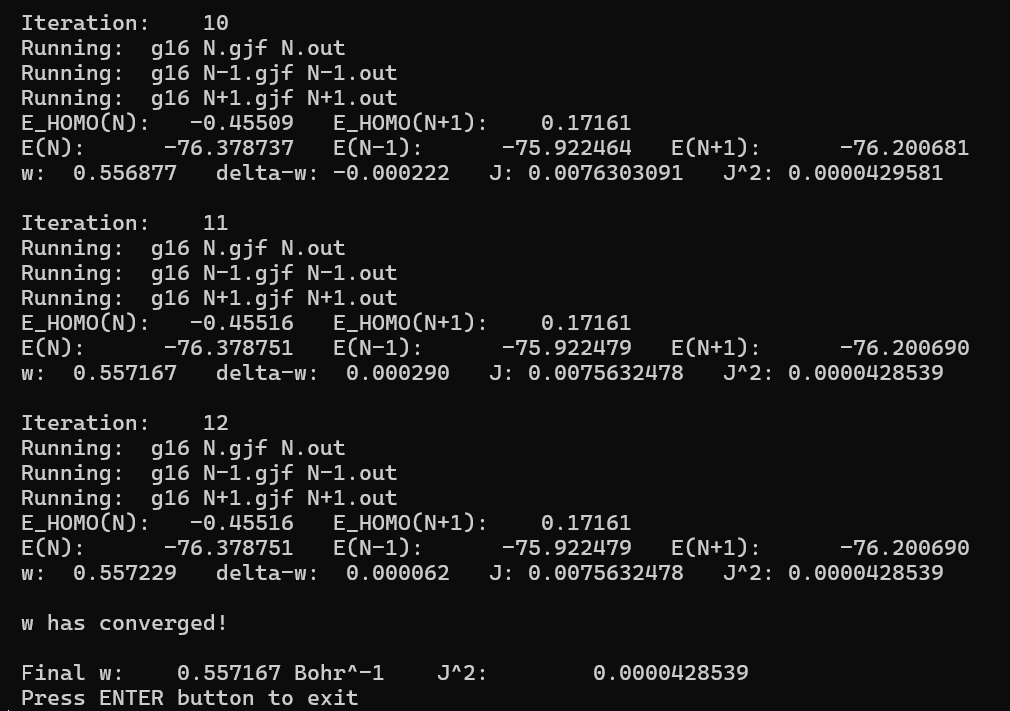
The output information is fully self-explanatory. Screenshot of final part of a very typical case is shown below:
It is noted that you can also run optDFTw in this way: optDFTw [wlow] [whigh] [winit] [wtol], the options given as arguments will overwite those in settings.ini. For example: ./optDFTw 0.2 0.5 0.39.
6When optimal ω is obtained using optDFTw, you can use it in practical calculations. For example, assume that the optimal value is 0.33, you should write keywords like follows:
-
Gaussian users:
# LC-wPBE/def2TZVP IOp(3/107=0330000000,3/108=0330000000)
-
ORCA users:
! LC-BLYP def2-tzvp tightSCF
%method  rangesepmu=0.33 end
Usage of scanDFTw
The use of scanDFTw is very similar with optDFTw, most settings in settings.ini as well as template file are the same, the only differences are:
- Executable files are
scanDFTw.exe(Windows) andscanDFTw(Linux) - In
settings.iniyou should setscanlow,scanhigh,scanstep, which correspond to lower limit (initial value), upper limit and stepsize of ω scan, respectively. You can also directly specify them as arguments, for example:./scanDFTw 0.1 0.8 0.05 1(the last "1" corresponds to "idetail" parameter)
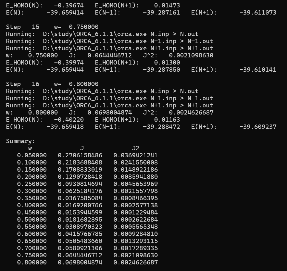
The output information is fully self-explanatory. Screenshot of final part of a very typical case is shown below: