Multiwfn forum
Multiwfn official website: http://sobereva.com/multiwfn. Multiwfn forum in Chinese: http://bbs.keinsci.com/wfn
You are not logged in.
- Topics: Active | Unanswered
Pages: 1
#1 Re: Multiwfn and wavefunction analysis » Multiwfn AdNDP Analysis with ORCA Output File » 2026-07-07 01:10:59
I'm posting my reply here for future user with the same question to see the results.
I used the phenanthrene molecule from section 4.14.3 in the Multiwfn manual and compared what I believe is the same calculation in ORCA. For others to see, here is the input file for the Gaussian calculation:
# b3lyp/3-21g pop=nboread
b3lyp/3-21g opted
0 1
C 0.00000000 3.56061700 -0.29722900
C 0.00000000 2.83932500 0.87979300
C 0.00000000 1.42361400 0.86771500
C 0.00000000 0.72986200 -0.38070000
C 0.00000000 1.49924400 -1.56931800
C 0.00000000 2.88151800 -1.53149000
C 0.00000000 0.67926500 2.09717700
C 0.00000000 -0.72986200 -0.38070000
C 0.00000000 -1.42361400 0.86771500
C 0.00000000 -0.67926500 2.09717700
C 0.00000000 -2.83932500 0.87979300
H 0.00000000 -3.34927800 1.83744900
C 0.00000000 -3.56061700 -0.29722900
C 0.00000000 -2.88151800 -1.53149000
C 0.00000000 -1.49924400 -1.56931800
H 0.00000000 1.23356400 3.02968400
H 0.00000000 4.64400700 -0.27588200
H 0.00000000 3.34927800 1.83744900
H 0.00000000 1.00203800 -2.53051300
H 0.00000000 3.44643700 -2.45642700
H 0.00000000 -1.23356400 3.02968400
H 0.00000000 -4.64400700 -0.27588200
H 0.00000000 -3.44643700 -2.45642700
H 0.00000000 -1.00203800 -2.53051300
$nbo dmnao aonao $end
And here is the input for the ORCA calculation:
! B3LYP 3-21G NBO
%nbo
nbokeylist="$nbo aonao dmnao $end"
end
%MaxCore 7500
%pal nprocs 16
end
* xyz 0 1
C 0.00000000 3.56061700 -0.29722900
C 0.00000000 2.83932500 0.87979300
C 0.00000000 1.42361400 0.86771500
C 0.00000000 0.72986200 -0.38070000
C 0.00000000 1.49924400 -1.56931800
C 0.00000000 2.88151800 -1.53149000
C 0.00000000 0.67926500 2.09717700
C 0.00000000 -0.72986200 -0.38070000
C 0.00000000 -1.42361400 0.86771500
C 0.00000000 -0.67926500 2.09717700
C 0.00000000 -2.83932500 0.87979300
H 0.00000000 -3.34927800 1.83744900
C 0.00000000 -3.56061700 -0.29722900
C 0.00000000 -2.88151800 -1.53149000
C 0.00000000 -1.49924400 -1.56931800
H 0.00000000 1.23356400 3.02968400
H 0.00000000 4.64400700 -0.27588200
H 0.00000000 3.34927800 1.83744900
H 0.00000000 1.00203800 -2.53051300
H 0.00000000 3.44643700 -2.45642700
H 0.00000000 -1.23356400 3.02968400
H 0.00000000 -4.64400700 -0.27588200
H 0.00000000 -3.44643700 -2.45642700
H 0.00000000 -1.00203800 -2.53051300
*
In the Multiwfn manual, the residual density distribution after accepting the first 27 orbitals is:
1 C : 1.0250 2C : 1.0370 3C : 1.0280 4C : 1.0414
5 C : 1.0339 6C : 1.0262 7C : 0.1322 8C : 1.0414
9 C : 1.0280 10C : 0.1322 11C : 1.0370 12H : 0.0117
13C : 1.0250 14C : 1.0262 15C : 1.0339 16H : 0.0121
17H : 0.0113 18H : 0.0117 19H : 0.0126 20H : 0.0111
21H : 0.0121 22H : 0.0113 23H : 0.0111 24H : 0.0126
In my ORCA calculations, I receive the following:
1C : 1.0234 2C : 1.0295 3C : 1.0243 4C : 1.0381
5C : 1.0246 6C : 1.0246 7C : 0.1302 8C : 1.0473
9C : 1.0167 10C : 0.1341 11C : 1.0345 12H : 0.0112
13C : 1.0234 14C : 1.0246 15C : 1.0217 16H : 0.0115
17H : 0.0106 18H : 0.0112 19H : 0.0120 20H : 0.0104
21H : 0.0115 22H : 0.0106 23H : 0.0104 24H : 0.0120
Later, the analysis of orbital 31 shows the following in the Multiwfn manual:
NAO# Center Label Type Composition
67 8(C ) px Val( 2p) 2.247%
76 9(C ) px Val( 2p) 1.929%
94 11(C ) px Val( 2p) 13.276%
105 13(C ) px Val( 2p) 32.846%
114 14(C ) px Val( 2p) 34.484%
123 15(C ) px Val( 2p) 15.204%
In my ORCA calculations, I receive the following:
NAO# Center Label Type Composition
67 8(C ) px Val( 2p) 2.217%
76 9(C ) px Val( 2p) 1.942%
94 11(C ) px Val( 2p) 13.387%
105 13(C ) px Val( 2p) 32.956%
114 14(C ) px Val( 2p) 34.401%
123 15(C ) px Val( 2p) 15.082%
As you can see, the differences between the two calculations in not very significant (>0.2 %); however, the visualization of the orbitals is still weird.
These are the orbitals from the Multiwfn manual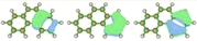
And here are the orbitals from my calculation (using a contour value of 0.03)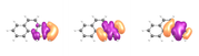
#2 Re: Multiwfn and wavefunction analysis » Multiwfn AdNDP Analysis with ORCA Output File » 2026-07-01 12:18:54
Thank you for the response, this was helpful.
I have one more question. Do you expect the composition of the AdNDP orbitals (i.e., for the O-H bond in water: %O composition, %2s/2p composition) to be reliable from an ORCA+NBO output file? I am currently working with an organometallic complex (optimized in ORCA followed by an NBO calculation in ORCA) and need to extract information about the polarization and hybridization of the metal-ligand bond.
#3 Multiwfn and wavefunction analysis » Multiwfn AdNDP Analysis with ORCA Output File » 2026-06-29 17:56:08
- b322qr
- Replies: 4
I am performing AdNDP analysis on molecules using option 14 in Multiwfn. I am performing the NBO calculation using ORCA and using the .out file as the input to Multiwfn. Everything works fine at this point. I can get the 1-center, 2-center, etc orbitals with what seems like the correct occupation numbers and %contributions from each participating atom. Then, when I want to visualize AdNDP analysis orbitals (using option 9 from the AdNDP submenu) from an NBO output file from an ORCA calculation, I create a .fch file by first making a .molden.input file and then converting it to a .fch file using option 100 then option 2 then option 7 in Multiwfn. However, the visualized orbitals are very weird. They do not look like typical orbitals you would expect. Even the O-H bond in water has an odd shape, which is totally delocalized over the entire molecule, that is not what you would expect from AdNDP analysis. I also have access to Gaussian and have run NBO calculations in Gaussian and performed AdNDP analysis with no problem.
Is there any way to fix this problem with ORCA? Is there a known workaround other than resorting to Gaussian?
#4 Re: Multiwfn and wavefunction analysis » sobEDA Unstable Wavefunction » 2024-08-09 12:38:02
Thank you, professor Lu. I appreciate your offer for help. I'm grateful that your code already creates the checkpoint file for each step of the calculation, making this process much easier. I would like your insight on my logic as I try to understand how to use the energy from the stable wavefunction to extract the information necessary for EDA. Most importantly, the "final" file.
I see at the bottom of the sobEDA.sh script that the only energy values that depend on the final energy are the total (dE_tot), dispersion (dE_disp), Pauli repulsion energy (dE_rep), and orbital energy (dE_orb). For reference, these are the lines of code I am looking at in the sobEDA.sh script.
##### Show summary of interaction #####
dE_tot=$E_tot_final
dE_els=$E_els_promol
dE_x=$E_x_promol
dE_c=$E_c_promol
dE_disp=$E_disp_final
for ((i=1;i<=$nfrag;i=i+1))
do
dE_tot=`echo "$dE_tot-(${E_tot[$i]})" | bc -l`
dE_els=`echo "$dE_els-(${E_els[$i]})" | bc -l`
dE_x=`echo "$dE_x-(${E_x[$i]})" | bc -l`
dE_c=`echo "$dE_c-(${E_c[$i]})" | bc -l`
dE_disp=`echo "$dE_disp-(${E_disp[$i]})" | bc -l`
done
dE_orb=`echo "$E_tot_final-($E_tot_frz)" | bc -l`
dE_rep=`echo "$E_tot_frz-($E_tot_promol)" | bc -l`
The final total energy (E_tot_final) looks for the energy in the line that says "SCF Done" in final.out, dispersion energy (E_disp_final) looks for the energy in the line that says "Dispersion energy" in final.out, frozen energy (E_tot_frz) looks for the energy shown in the first cycle in final.out (which final.gjf reads from the promol.chk file), and E_tot_promol looks for the energy in the line that says "SCF Done" in promol.out.
After running a single point calculation (let's call this new single point calculation "final2") using the same route section as final.gjf, but reading the guess from the stable wavefunction, I receive an output that finishes after only 1 cycle (I guess because it is reading from an already optimized, stable wavefunction). With the knowledge of the way the parameters of EDA are calculated by the program, I compare between final and final2 the dispersion energy (it does not change, and therefore dE_disp would not change) and the final energy printed after "SCF Done" (it becomes more negative because of the stable wavefunction).
If I try to perform the EDA on final2.out, obviously I will get erroneous results because the frozen energy is the same as the final energy (it finishes in one cycle). So, my next thought is to modify the line in the original final.out that says "SCF Done" and replace it with the energy from that same line in final2.out. (i.e. change "SCF Done: E(UPBE1PBE) = XXX.XXX" to " SCF Done: E(UPBE1PBE) = YYY.YYY") That way the final energy represents the energy from the stable wavefunction. Although, this is assuming the frozen energy would remain the same.
Please let me know if my logic is correct and if it is reasonable to replace the energy value shown after "SCF Done" in final.out with the energy from final2.out.
#5 Multiwfn and wavefunction analysis » sobEDA Unstable Wavefunction » 2024-07-29 15:15:05
- b322qr
- Replies: 3
I am using sobEDA on an actinide system and after it has completed, I run a stability check in Gaussian using the "final.chk" checkpoint file, which then shows that the calculation has an unstable wavefunction. What should I do in order to get the correct energy decomposition analysis with the stable wavefunction? Would I be able to run another second single point calculation using the stable wavefunction as a guess wavefunction and extract the EDA parameters from there?
#6 Re: Multiwfn and wavefunction analysis » Saving AdNDP Results to a Text File » 2024-05-06 14:37:58
Thank you! This solves my issue.
#7 Re: Multiwfn and wavefunction analysis » Saving AdNDP Results to a Text File » 2024-05-03 19:34:54
Thank you, professor Lu. I am curious if there is a way to write this in a bash script for Linux operating system. I would like to automate this process.
#8 Multiwfn and wavefunction analysis » Saving AdNDP Results to a Text File » 2024-05-02 18:27:45
- b322qr
- Replies: 4
In the AdNDP analysis module, is it possible to take the composition of candidate orbitals and export them to a text file for further analysis of data?
For example, I start with an NBO.log file, go to the AdNDP module, and perform an exhaustive search for 1c and 2c orbitals. I pick out the first 3 candidate orbitals for the 2c orbitals and then evaluate them using option 15 "Evaluate and output composition of AdNDP orbitals". From there, the contribution from each atom and shell can be found. This is the information that I would like to save in a text file. I have a repetitive task where I obtain and pick out the atom contribution and shell contribution data manually and put it into a spreadsheet. I would like to make code to do this automatically, but I know of no way to output this data in a text file.
#9 Re: Multiwfn and wavefunction analysis » Issue with saving graph to image file using a batch script » 2024-05-01 12:01:30
Ah, I see, I was using the noGUI version of Multiwfn. Thank you very much.
#10 Multiwfn and wavefunction analysis » Issue with saving graph to image file using a batch script » 2024-04-30 13:07:07
- b322qr
- Replies: 2
I am trying to automate the process of generating an image file for DOS plots by using batch scripting. Below are the two files I am using, DOS.sh and DOS.txt. When I run the script, the DOS_line.txt and DOS_curve.txt files are generated as expected, but the image file containing the graph is not. How should I modify the script to output the image file in the current working directory?
DOS.sh
////////////////////////////////////////////////
#!/bin/bash
for inf in *.fchk
do
Multiwfn ${inf} <DOS.txt> /dev/null
mv -f DOS_line.txt ${inf//fchk}_line.txt
mv -f DOS_curve.txt ${inf//fchk}_curve.txt
done
////////////////////////////////////////////////
DOS.txt
////////////////////////////////////////////////
10
8
0
3
2
0
-10
////////////////////////////////////////////////
Pages: 1